Examples

There are numerous resources that you might find useful for learning and using badlands.

The following set of notebooks go through the main workflows for constructing and running surface processes models. These models demonstrate badlands current best usage practises, and are guaranteed to operate correctly for each badlands release.

They are available as a github repository.

git clone https://github.com/badlands-model/badlands-workshop.git

Required Python Skills

To use badlands successfully, you will need to have an understanding of the following Python constructs:

1. Basic Python, such as importing modules, and syntax structure (indenting, functions, etc).
2. Containers such as dictionaries, lists and tuples.
3. Flow control (loops, if-else conditionals, etc).
4. Python objects, object methods, object attributes, object lifecycles.

Most beginner (or intermediate) Python tutorials should cover these concepts.

Badlands uses h5py for all heavy data disk IO. H5py is a Python library which provides a Python interface to writing/reading HDF5 format files. While not strictly required, more advanced users will certainly find having some familiarity with the h5py libary useful, both for directly querying files badlands has generated, and also for writing their own files (in preference to CSV for example).

Jupyter Notebooks

Jupyter Notebooks is the recommended environment for most model development. In badlands we utilise notebooks to provide inline visualisation of your model configurations, allowing you to quickly see your results, modify as required, and then regenerate and repeat.

If you are new to Jupyter Notebooks, you should familiarise yourself with the notebook environment first. Also, remember the Help menu bar option provides useful references and keyboard shortcuts.

How to get help

If you encounter issues or suspect a bug, please create a ticket using the issue tracker on github.

Testing models

A series of examples are available with the source code. These examples illustrate the different capabilities of the code and are an ideal starting point to learn how to use badlands. Each folder is composed of

1. an input XML file where the different options for the considered experiment are set,
2. a data folder containing the initial surface and potentially some forcing files (e.g. sea-level, rainfall or tectonic grids) and
3. a series of IPython notebooks used to run the experiment and perform some pre or post-processing tasks.

Tip

These examples have been designed to be run quickly and should take on average 5 minutes on standard computer.

Table 1 Summary of hands-on examples provided with badlands package. Abbreviations: dim.: model dimension – rain uni./oro.: uniform or orographic – res.: model resolution – fluv.: fluvial processes – hillslp.: hillslope – strat.: stratigraphic architecture – s.l.: sea-level – tect.: tectonics.

Exp.	dim. [km]	res.	time	Forcings & Processes
Basin	30 x 30	100 m	1 Ma	Rain uni. | Fluv./hillslp. | s.l. | Strat.
Crater	2.5 x 2.5	10 m	200 ka	Rain uni. | Fluv./hillslp.
Delta	25 x 25	50 m	500 ka	Rain uni. | Fluv./hillslp. | s.l. | tect. | Strat.
Dyntopo	300 x 200	1 km	10 Ma	Rain uni. | Fluv./hillslp. | s.l.
eTopo	133 x 180	50 m	500 ka	Rain uni. | Fluv./hillslp. | s.l. | tect.
Flexure	250 x 100	500 m	1 Ma	Rain uni. | Fluv./hillslp. | gflex
Mountain	80 x 40	400 m	10 Ma	Rain oro. | Fluv./hillslp.
Rift	400 x 400	2 km	250 ka	Rain uni. | Fluv./hillslp. | 3D tect.
Strikeslip	200 x 200	1 km	100 ka	Rain uni. | Fluv./hillslp. | 3D tect.

The range of simulations varies both in term of spatial and temporal resolutions. A summary of the proposed models is presented in Table 1 and could serve as a basis for more complex problems. You can browse the list of examples directly from the IPython notebooks.

Companion

To assist users during the pre and post-processing phases, a series of Python classes are proposed in a GitHub badlands-companion repository. These classes are shipped with the Docker container mentioned in previous section. In addition, IPython notebooks have been created to illustrate how these python classes are used. We have chosen this structure to give users the transparency and opportunity to

1. clearly understand the creation and format of the input files,
2. perform quantitative analyses of badlands output files,
3. easily design their own notebooks and further improve the proposed workflow.

To install the companion functions on your local environment, we provide a Python Package:

pip install badlands-companion

In case where the installation does not work, a local installation can be done:

git clone https://github.com/badlands-model/badlands-companion.git
cd badlands-companion
python3 setup.py install

Pre-processing classes

The pre-processing notebooks allows for quick creation of grids and files compatible with badlands input format. The main functionalities and associated notebook filenames are listed below:

• topographic grids for generic model (topoCreate),
• real topographic/bathymetric dataset (etopoGen),
• building sea level fluctuations curve or using Haq curve (seaLevel),
• horizontal displacement and precipitation maps (topoTec),
• regridding initial tectonic, rainfall and topographic input files (regridInput)

Post-processing classes

Morphometric & Hydrometric

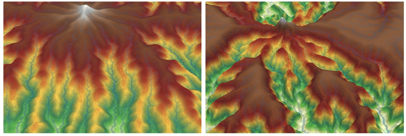
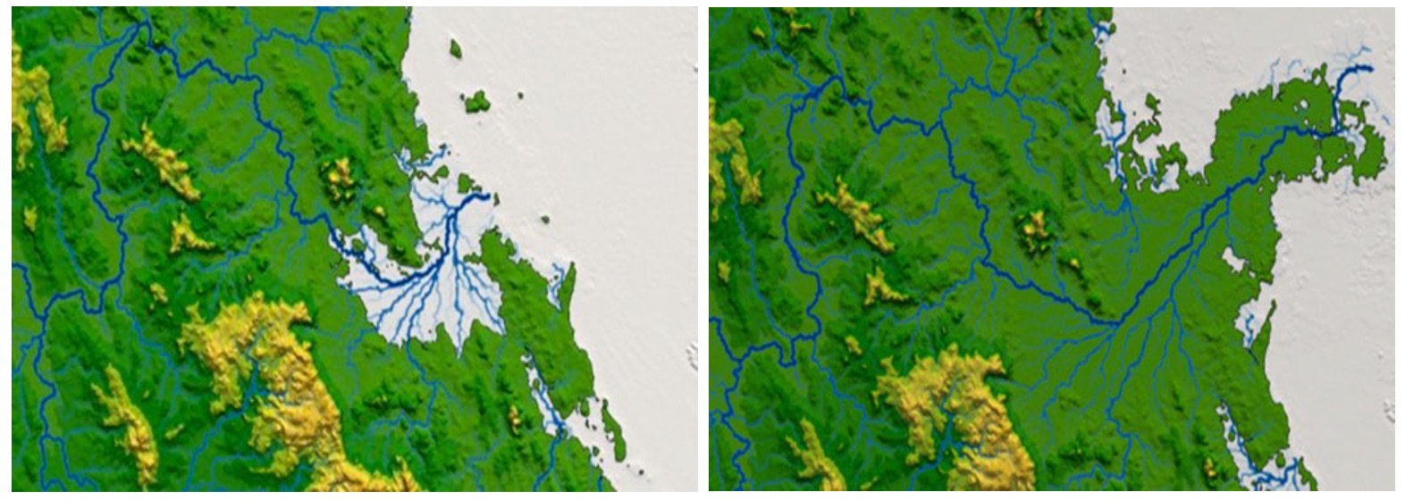
The morphometrics notebook can be used to perform quantitative analyses of simulated badlands landforms [1] [2]. Gradients, curvature (horizontal and vertical), aspect and discharge attributes can be extracted for the entire region or a specific area of the simulation. The hydrometric notebook allows for evaluation of time dependent evolution of a specific catchment. It can be used to quantify the longitudinal evolution of a river profile, compute the Peclet number distribution, \(\chi\)-maps as well as hypsometric curves.

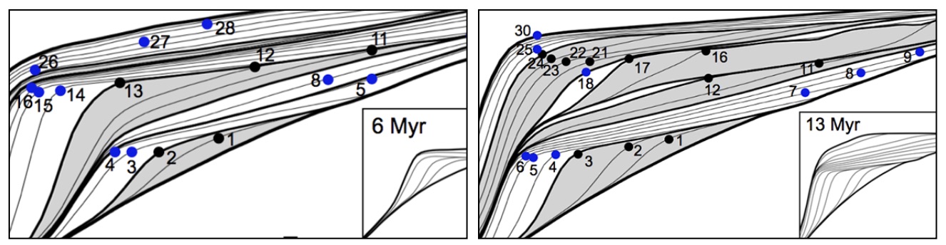
Stratigraphy & Wheeler diagram

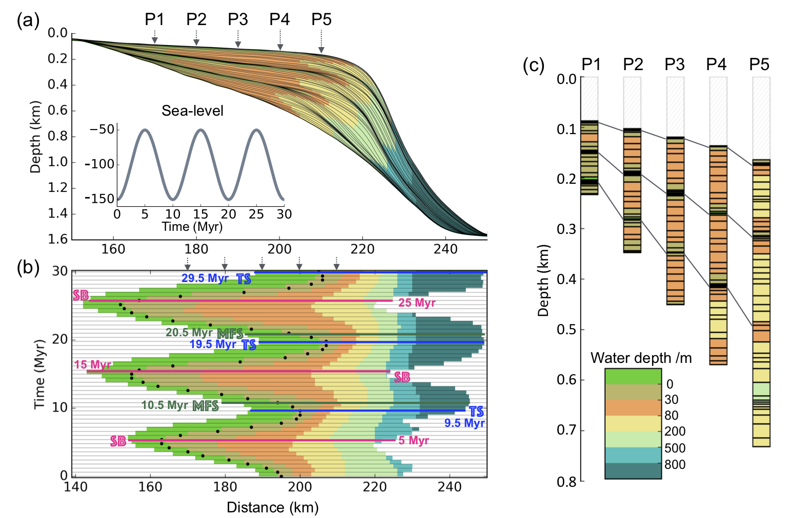
Fig. 1 Predicted stratal architecture. (a) Stratal stacking patterns on a vertical cross-section. Solid black lines shown on each subplot are stratigraphic layers and are plotted at 0.5 Myr intervals. The coupled sea-level scenario is modelled as a sinusoidal curve. Different colours stand for different depositional environments that are defined based on water depth. (b) Wheeler diagram or chronostratigraphy chart. The black dots are shoreline positions through time, or shoreline trajectory. The coloured dashed lines are stratigraphic surfaces identified based on stratal terminations, stacking trends and shoreline trajectory. (c) Virtual cores extracted at different positions: P1, P2, P3, P4, P5. Solid lines connect condensed sections that are associated with unconformity due to sea-level fall.

When the stratigraphic structure is turned on in badlands, it is possible to extract cross-section and plot stratigraphic layers, Wheeler diagram and virtual cores. The notebook extracts simulated depositional sequences on a vertical cross-section, and calculates the relative sea level change, shoreline trajectory, accommodation and sedimentation change. Three methods can be applied to interpret the stratigraphic units including

• the systems tracts model based on relative sea level change,
• the shoreline trajectory analysis [3] and
• the accommodation succession method [4] [5].

Using the stratalMesh notebook, it is also possible to export the simulated stratigraphy as a VTK structured mesh that could be further analysed in other software packages.

Workshop

A set of workshop documents and models are also provided and aims to introduce those interested in landscape evolution and source to sink problems to badlands.

The set of problems is quite broad and should be of interest to a wide community. The workshop as been designed to run over a couple of days but can be shorten if needed!

Note

You do not have to be a seasoned modeller to participate. Geomorphologists, tectonicists and sedimentologists interested in testing conceptual models based on field observations are welcome!

We welcome all kinds of contributions! Please get in touch if you would like to help out.

Important

Everything from code to notebooks to examples and documentation are all equally valuable so please don’t feel you can’t contribute.

To contribute please fork the project make your changes and submit a pull request. We will do our best to work through any issues with you and get your code merged into the main branch.

If you found a bug, have questions, or are just having trouble with badlands, you can:

• join the badlands User Group on Slack by sending an email request to: tristan.salles@sydney.edu.au
• open an issue in our issue-tracker and we’ll try to help resolve the concern.

---

[1]	T. Salles and L. Hardiman - Badlands: An open-source, flexible and parallel framework to study landscape dynamics, Computers & Geosciences, vol. 91, no. Supplement C, pp. 77–89, 2016.

[2]	T. Salles, N. Flament, and D. Müller - Influence of mantle flow on the drainage of eastern Australia since the jurassic period, Geochemistry, Geophysics, Geosystems, vol. 18, no. 1, pp. 280–305, 2017.

[3]	W. Helland-Hansen and G. Hampson - Trajectory analysis: concepts and applications, Basin Research, vol. 21, no. 5, pp. 454–483, 2009.

[4]	J. Neal and V. Abreu - Sequence stratigraphy hierarchy and the accommodation succession method, Geology, vol. 37, no. 9, pp. 779–782, 2009.

[5]	J. E. Neal, V. Abreu, K. M. Bohacs, H. R. Feldman, and K. H. Pederson - Accommodation succession (δa/δs) sequence stratigraphy: observational method, utility and insights into sequence boundary formation, Journal of the Geological Society, vol. 173, no. 5, pp. 803–816, 2016.