API Documentation¶

Badlands is a long-term surface evolution model built to simulate landscape development, sediment transport and sedimentary basins formation from upstream regions down to marine environments.

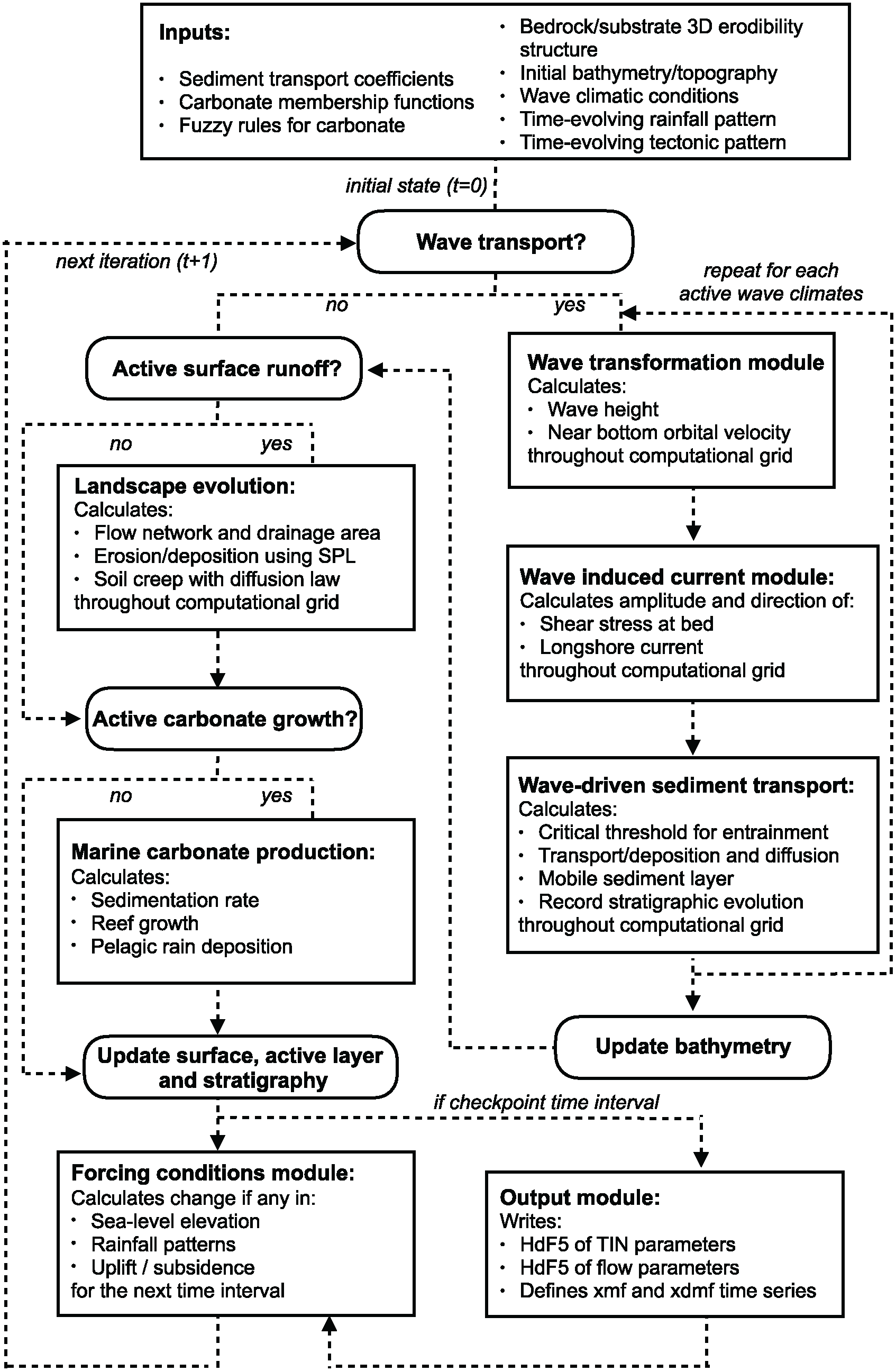
The above figure illustrates the relationships between the different modules of the framework.

Below you will find the nitty-gritty components of the Python code… The following API documentation provides a nearly complete description of the different functions that compose the code… ✌️

Warning

It is worth mentioning that a set of fortran & C functions are also part of badlands code but are not described in this API…

Model class¶

Main components of badlands workflow.

class model.Model[source]¶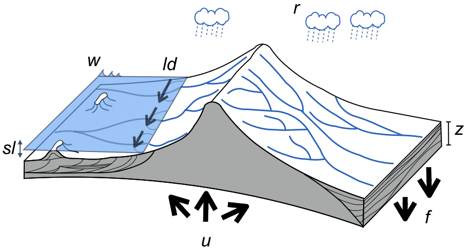

A schematic of badlands capabilities illustrating the main variables and forcing conditions. w represents the wave boundary conditions, ld the longshore drift, sl the sea-level, u the tectonic, f the flexural isostasy and r the rainfall patterns. The stratigraphic evolution and morphology are computed through time.

Tip

If you are not intending to develop new functionalities, the following two functions are the main ways to interact with badlands and are probably all you need to know about the API documentation 💥 ✌️

load_xml(filename, verbose=False)[source]¶

Load the XML input file describing the experiment parameters.

Parameters:	filename – (str) path to the XML file to load. verbose – (bool) when `True`, output additional debug information (default: `False`).

Note

Additional information regarding the input file XML options are found on badlands website.
A good way to start learning badlands consists in running the Jupyter Notebooks examples.

run_to_time(tEnd, verbose=False)[source]¶

Run the simulation to a specified point in time.

Parameters:	tEnd – (float) time in years up to run the model for… verbose – (bool) when `True`, output additional debug information (default: `False`).

Warning

If specified end time (tEnd) is greater than the one defined in the XML input file priority is given to the XML value.

Flow Network¶

Implementation related to badlands flow network algorithm.

flowNetwork¶

This file defines functions to compute stream network over the TIN.

class flow.flowNetwork.flowNetwork(input)[source]¶

Class used to define flow network computation.

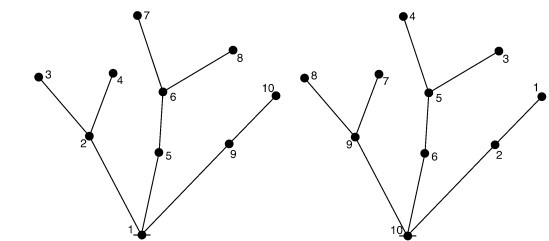
The left graph shows the stack order considering the single-flow-direction algorithm and the right graph shows the inverted stack order from top to bottom as described in Braun and Willett (2013).

See also

Braun J, Willett SD. A very efficient O(n), implicit and parallel method to solve the stream power equation governing fluvial incision and landscape evolution. Geomorphology. 2013;180–181(Supplement C):170–179.

compute_failure(elev, sfail)[source]¶

Perform erosion induced by slope failure.

Parameters:

elev – numpy arrays containing the elevation of the TIN nodes.
sfail – critical slope to initiate slope failure.

Returns:

erosion - numpy integer-type array containing for local nodes their global IDs.

compute_failure_diffusion(elev, depoH, neighbours, edges, distances, coeff, globalIDs, maxth, tstep)[source]¶

Perform slope failure transported sediments diffusion.

Parameters:

elev – numpy arrays containing the elevation of the TIN nodes.
dep – numpy arrays flagging the deposited nodes.
neighbours – numpy integer-type array with the neighbourhood IDs.
edges – numpy real-type array with the voronoi edges length for each neighbours of the TIN nodes.
distances – numpy real-type array with the distances between each connection in the TIN.
globalIDs – numpy integer-type array containing for local nodes their global IDs.

Returns:

diff_flux – numpy array containing erosion/deposition thicknesses induced by slope failure processes.
mindt – maximum time step (in years) to ensure stable results

compute_flow(sealevel, elev, Acell, rain)[source]¶

Calculates the drainage area and water discharge at each node.

Parameters:	elev – numpy arrays containing the elevation of the TIN nodes. Acell – numpy float-type array containing the voronoi area for each nodes (in \({m}^2\)). rain – numpy float-type array containing the precipitation rate for each nodes (in \({m/a}\)).

compute_hillslope_diffusion(elev, neighbours, edges, distances, globalIDs, type, Sc)[source]¶

Perform hillslope evolution based on diffusion processes.

Parameters:

elev – numpy arrays containing the elevation of the TIN nodes.
neighbours – numpy integer-type array with the neighbourhood IDs.
edges – numpy real-type array with the voronoi edges length for each neighbours of the TIN nodes.
distances – numpy real-type array with the distances between each connection in the TIN.
globalIDs – numpy integer-type array containing for local nodes their global IDs.
type – flag to compute the diffusion when multiple rocks are used.
Sc – critical slope parameter for non-linear diffusion.

Returns:

diff_flux - numpy array containing erosion/deposition thicknesses induced by hillslope processes.

compute_marine_diffusion(elev, depoH, neighbours, edges, distances, coeff, globalIDs, seal, maxth, tstep)[source]¶

Perform river transported marine sediments diffusion.

Parameters:

elev – numpy arrays containing the elevation of the TIN nodes.
dep – numpy arrays flagging the deposited nodes.
neighbours – numpy integer-type array with the neighbourhood IDs.
edges – numpy real-type array with the voronoi edges length for each neighbours of the TIN nodes.
distances – numpy real-type array with the distances between each connection in the TIN.
globalIDs – numpy integer-type array containing for local nodes their global IDs.

Returns:

diff_flux – numpy array containing marine erosion/deposition thicknesses induced by hillslope processes.
mindt – maximum time step (in years) to ensure stable results

compute_parameters(elevation, sealevel)[source]¶: Calculates the catchment IDs and the Chi parameter (Willett 2014).

compute_parameters_depression(fillH, elev, Acell, sealevel, debug=False)[source]¶

Calculates each depression maximum deposition volume and its downstream draining node.

Parameters:	fillH – numpy array containing the filled elevations from Planchon & Darboux depression-less algorithm. elev – numpy arrays containing the elevation of the TIN nodes. Acell – numpy float-type array containing the voronoi area for each nodes (in \({m}^2\)) sealevel – real value giving the sea-level height at considered time step.

compute_sedflux(Acell, elev, rain, fillH, dt, actlay, rockCk, rivqs, sealevel, perc_dep, slp_cr, ngbh, verbose=False)[source]¶

Calculates the sediment flux at each node.

Parameters:

Acell – numpy float-type array containing the voronoi area for each nodes (in \({m}^2\))
elev – numpy arrays containing the elevation of the TIN nodes.
rain – numpy float-type array containing the precipitation rate for each nodes (in \({m/a}\)).
fillH – numpy array containing the lake elevations.
dt – real value corresponding to the maximal stability time step.
actlay – active layer composition.
rockCk – rock erodibility values.
rivqs – numpy arrays representing the sediment fluxes from rivers.
sealevel – real value giving the sea-level height at considered time step.
slp_cr – critical slope used to force aerial deposition for alluvial plain.
perc_dep – maximum percentage of deposition at any given time interval.

Returns:

erosion – numpy array containing erosion thicknesses for each node of the TIN (in m).
depo – numpy array containing deposition thicknesses for each node of the TIN (in m).
sedflux – numpy array containing cumulative sediment flux on each node (in \({m}^3/{m}^2\)).
newdt – new time step to ensure flow computation stability.

compute_sediment_hillslope(elev, difflay, coeff, neighbours, edges, layh, distances, globalIDs)[source]¶

Perform sediment diffusion for multiple rock types.

Parameters:

elev – numpy arrays containing the elevation of the TIN nodes.
difflay – numpy arrays containing the rock type fractions in the active layer.
coeff – numpy arrays containing the coefficient value for the diffusion algorithm.
neighbours – numpy integer-type array with the neighbourhood IDs.
edges – numpy real-type array with the voronoi edges length for each neighbours of the TIN nodes.
layh – numpy arrays containing the thickness of the active layer.
distances – numpy real-type array with the distances between each connection in the TIN.
globalIDs – numpy integer-type array containing for local nodes their global IDs.

Returns:

ero – 2D numpy array containing erosion thicknesses for each sediment diffused by hillslope processes.
depo – 2D numpy array containing deposition thicknesses for each sediment diffused by hillslope processes.
sumdiff – numpy array containing cumulative erosion/deposition thicknesses induced by hillslope processes.

compute_sediment_marine(elev, dep, sdep, coeff, neighbours, seal, maxth, edges, distances, globalIDs)[source]¶

Perform marine sediment diffusion for multiple rock types.

Parameters:

elev – numpy arrays containing the elevation of the TIN nodes.
dep – numpy arrays containing the rock deposition.
coeff – numpy arrays containing the coefficient value for the diffusion algorithm.
neighbours – numpy integer-type array with the neighbourhood IDs.
edges – numpy real-type array with the voronoi edges length for each neighbours of the TIN nodes.
distances – numpy real-type array with the distances between each connection in the TIN.
globalIDs – numpy integer-type array containing for local nodes their global IDs.

Returns:

diff_prop – 2D numpy array containing proportion of each sediment diffused by marine processes.
diff_flux – numpy array containing erosion/deposition thicknesses induced by marine processes.

dt_stability(elev, locIDs)[source]¶

This function computes the maximal timestep to ensure computation stability of the flow processes.

Important

This CFL-like condition is computed using:

erodibility coefficients,
discharge and elevation and
distances between TIN nodes donors and receivers.

Parameters:	elev – numpy arrays containing the elevation of the TIN nodes. locIDs – numpy integer-type array containing local nodes global IDs.

ordered_node_array_elev()[source]¶: Creates an array of node IDs that is arranged in order from downstream to upstream for real surface.

ordered_node_array_filled()[source]¶: Creates an array of node IDs that is arranged in order from downstream to upstream for filled surface.

view_receivers(fillH, elev, neighbours, edges, distances, globalIDs, sea)[source]¶

Single Flow Direction function computes downslope flow directions by inspecting the neighborhood elevations around each node. The SFD method assigns a unique flow direction towards the steepest downslope neighbor.

Parameters:

fillH – numpy array containing the filled elevations from Planchon & Darboux depression-less algorithm.
elev – numpy arrays containing the elevation of the TIN nodes.
neighbours – numpy integer-type array with the neighbourhood IDs.
edges – numpy real-type array with the voronoi edges length for each neighbours of the TIN nodes.
distances – numpy real-type array with the distances between each connection in the TIN.
globalIDs – numpy integer-type array containing for local nodes their global IDs.
sea – current elevation of sea level.

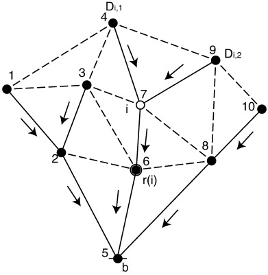
Nodal representation of the landform. Nodes are indicated as black circles. The lines represent all the possible connections among neighboring nodes. The solid lines indicate the connections following the steepest descent hypothesis (indicated by the arrows).

visualiseFlow¶

The set of functions below are used to export the flow network and the associated variables computed with badlands.

Badlands uses `hdf5`_ library for outputs generation. To read the hdf5 files, the code creates a XML schema (.xmf files) describing how the data is stored in the hdf5 files.

Then `xdmf`_ files provides support to visualise temporal evolution of the output with applications such as Paraview or Visit.

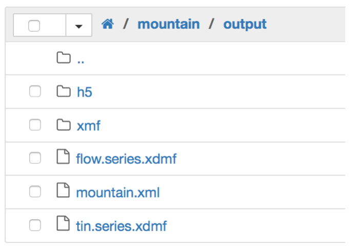
Above is a typical structure that you will find in badlands output folder:

h5 folder contains the hdf5 data, all the information computed by the model are stored in these files. You will have at least the tin (surface) and flow (stream network) dataset and also the sed (stratigraphy) data if the stratal structure is computed in your simulation.
xmf folder contains the XML files used to read the hdf5 files contained in the h5 folder.
the .xml input file used to build this specific model.
two .xdmf files for the surface (tin_series.xdmf) and the flow network (flow_series.xdmf) that read the xmf files through time.

Important

The flow outputs are hdf5 files.

flow.visualiseFlow.output_Polylines(outPts, rcvIDs, visXlim, visYlim, coordXY)[source]¶

This function defines the connectivity array for visualising flow network.

Parameters:

outPts – numpy integer-type array containing the output node IDs.
inIDs – numpy integer-type local nodes array filled with global node IDs excluding partition edges.
visXlim – numpy array containing the X-axis extent of visualisation grid.
visYlim – numpy array containing the Y-axis extent of visualisation grid.
coordXY – 2D numpy float-type array containing X, Y coordinates of the local TIN nodes.

Returns:

flowIDs – numpy integer-type array containing the output node IDs for the flow network.
polyline – numpy 2D integer-type array containing the connectivity IDs for each polyline.

flow.visualiseFlow.write_hdf5(folder, h5file, step, coords, elevation, discharge, chi, sedload, flowdensity, basin, connect)[source]¶

This function writes for each processor the HDF5 file containing flow network information.

Parameters:

folder – name of the output folder.
h5file – first part of the hdf5 file name.
step – output visualisation step.
coords – numpy float-type array containing X, Y coordinates of the local TIN nodes.
elevation – numpy float-type array containing Z coordinates of the local TIN nodes.
discharge – numpy float-type array containing the discharge values of the local TIN.
chi – numpy float-type array containing the chi values of the local TIN.
sedload – numpy float-type array containing the sedload values.
flowdensity – numpy float-type array containing the flow density.
basin – numpy integer-type array containing the basin IDs values of the local TIN.
connect – numpy 2D integer-type array containing the local nodes IDs for each connected network.

flow.visualiseFlow.write_xmf(folder, xmffile, xdmffile, step, time, elems, nodes, h5file)[source]¶

This function writes the XmF file which is calling each hdf5 file.

Parameters:

folder – name of the output folder.
xmffile – first part of the XmF file name.
xdmffile – XDmF file name.
step – output visualisation step.
time – simulation time.
elems – numpy integer-type array containing the number of cells of each local partition.
nodes – numpy integer-type array containing the number of nodes of each local partition.
h5file – first part of the hdf5 file name.

Forcing¶

forceSim¶

carbGrowth¶

isoFlex¶

pelagicGrowth¶

xmlParser¶

Hillslope¶

Implementation related to badlands hillslope processes.

diffLinear¶

This module encapsulates functions related to badlands hillslope computation based on diffusion.

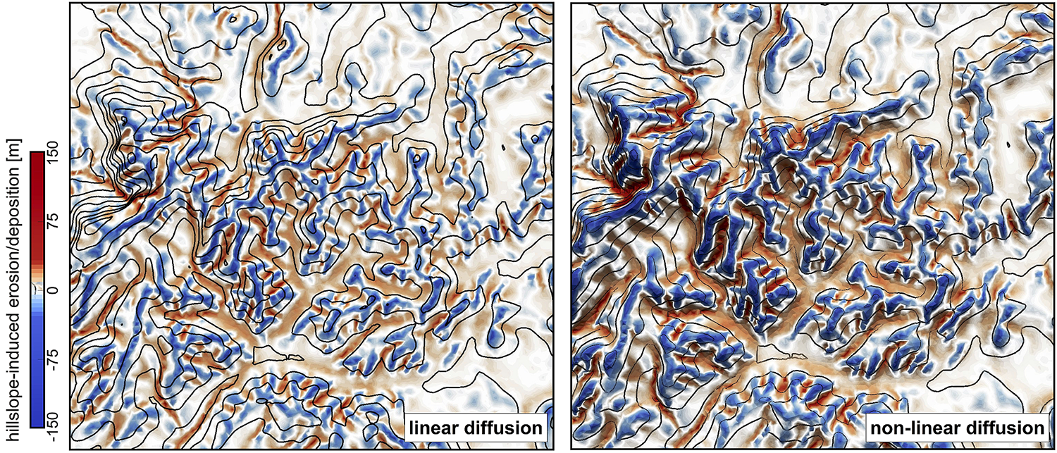
Erosion/deposition induced after 130 ka of hillslope diffusion using the linear and non-linear formulations. Left: Linear diffusion produces convex upward slopes (κhl = κhn = 0.05). Right: non-linear approach tends to have convex to planar profiles as hillslope processes dominate when slopes approach or exceed the critical slope (Sc = 0.8)

class hillslope.diffLinear.diffLinear[source]¶

Class for handling hillslope computation using a linear/non-linear diffusion equation.

dt_stability(edgelen)[source]¶

This function computes the maximal timestep to ensure computation stability of the hillslope processes. This CFL-like condition is computed using diffusion coefficients and distances between TIN nodes.

Note

It is worth noticing that the approach does not rely on the elevation of the nodes and therefore the maximal hillslope timestep to ensure stability just needs to be computed once for each given TIN grid.

Parameters:	edgelen – numpy array containing the edges of the TIN surface for the considered partition.

dt_stabilityCs(elev, neighbours, distances, globalIDs, borders)[source]¶

This function computes the maximal timestep to ensure computation stability of the non-linear hillslope processes.

Note

This CFL-like condition is computed using non-linear diffusion coefficients and distances between TIN nodes.

Parameters:	edgelen – numpy array containing the edges of the TIN surface for the considered partition. elevation – numpy array containing the edges of the TIN surface for the considered partition.

dt_stability_fail(edgelen)[source]¶

This function computes the maximal timestep to ensure computation stability of the slope failure processes. This CFL-like condition is computed using diffusion coefficients and distances between TIN nodes.

Parameters:	edgelen – numpy array containing the edges of the TIN surface for the considered partition.

dt_stability_ms(edgelen)[source]¶

This function computes the maximal timestep to ensure computation stability of the river deposited marine sediment processes. This CFL-like condition is computed using diffusion coefficients and distances between TIN nodes.

Note

It is worth noticing that the approach does not rely on the elevation of the nodes and therefore the maximal hillslope timestep to ensure stability just needs to be computed once for each given TIN grid.

Parameters:	edgelen – numpy array containing the edges of the TIN surface for the considered partition.

sedflux(sea, elevation, area)[source]¶

This function computes the sedimentary fluxes induced by hillslope processes based on a linear diffusion approximation.

Important

The linear diffusion process is implemented through the FV approximation and is based on the area of each node voronoi polygon and the sum over all the neighbours of the slope of the segment (i.e. height differences divided by the length of the mesh edge) as well as the length of the corresponding voronoi edge.

Parameters:

sea – float value giving the sea-level height at considered time step.
elevation – numpy array containing the edges of the TIN surface for the considered partition.
area – numpy array containing the area of the voronoi polygon for each TIN nodes.

Returns:

CA - numpy array containing the diffusion coefficients.

sedfluxfailure(area)[source]¶

This function computes the diffusion of slope failure using a linear diffusion approximation.

Parameters:	area – numpy array containing the area of the voronoi polygon for each TIN nodes.
Returns:	CA - numpy array containing the diffusion coefficients.

sedfluxmarine(sea, elevation, area)[source]¶

This function computes the diffusion of marine sediments transported by river processes using a linear diffusion approximation.

Parameters:

sea – float value giving the sea-level height at considered time step.
elevation – numpy array containing the edges of the TIN surface for the considered partition.
area – numpy array containing the area of the voronoi polygon for each TIN nodes.

Returns:

CA - numpy array containing the diffusion coefficients.

Simulation¶

Implementation related to badlands main simulation functions.

buildFlux¶

This file is the main entry point to compute flow network and associated sedimentary fluxes.

simulation.buildFlux.sediment_flux(input, recGrid, hillslope, FVmesh, flow, force, rain, lGIDs, applyDisp, straTIN, mapero, cumdiff, cumhill, cumfail, fillH, disp, inGIDs, elevation, tNow, tEnd, verbose=False)[source]¶

Compute sediment fluxes.

Parameters:

input – class containing XML input file parameters.
recGrid – class describing the regular grid characteristics.
hillslope – class describing hillslope processes.
FVmesh – finite volume mesh.
flow – flow parameters.
force – forcing parameters.
rain – rain values.
lGIDs – global nodes indices.
applyDisp – applying displacement boolean.
straTIN – class for stratigraphic TIN grid.
mapero – imposed erodibility maps.
cumdiff – cumulative total erosion/deposition changes.
cumhill – cumulative hillslope erosion/deposition changes.
cumfail – cumulative failure induced erosion/deposition changes.
fillH – filled elevation mesh.
disp – displacement values .
inGIDs – nodes indices.
elevation – elevation mesh
tNow – simulation time step.
tEnd – simulation end time.
verbose – (bool) when True, output additional debug information (default: False).

Returns:

tNow – simulation current time.
elevation – updated numpy 1D array containing the elevations.
cumdiff – updated cumulative total erosion/deposition changes
cumhill – updated cumulative hillslope erosion/deposition changes
cumfail – updated cumulative failure induced erosion/deposition changes

simulation.buildFlux.streamflow(input, FVmesh, recGrid, force, hillslope, flow, elevation, lGIDs, rain, tNow, verbose=False)[source]¶

Compute stream flow.

Parameters:

input – class containing XML input file parameters.
FVmesh – class describing the finite volume mesh.
recGrid – class describing the regular grid characteristics.
force – class describing the forcing parameters.
hillslope – class describing hillslope processes.
flow – class describing stream power law processes.
elevation – numpy array containing the elevations for the domain.
lGIDs – numpy 1D array containing the node indices.
rain – numpy 1D array containing rainfall precipitation values.
tNow – simulation time step.
verbose – (bool) when True, output additional debug information (default: False).

Returns:

fillH – numpy 1D array containing the depression-less elevation values.
elev – numpy 1D array containing the elevations.

buildMesh¶

This file defines the functions used to build badlands meshes and surface grids.

simulation.buildMesh.construct_mesh(input, filename, verbose=False)[source]¶

The following function is taking parsed values from the XML to:

build model grids & meshes,
initialise Finite Volume discretisation,
define the partitioning when parallelisation is enable.

Parameters:

input – class containing XML input file parameters.
filename – (str) this is a string containing the path to the regular grid file.
verbose – (bool) when True, output additional debug information (default: False).

Returns:

recGrid – class describing the regular grid characteristics.
FVmesh – class describing the finite volume mesh.
force – class describing the forcing parameters.
lGIDs – numpy 1D array containing the node indices.
fixIDs – numpy 1D array containing the fixed node indices.
inGIDs – numpy 1D array containing the node indices inside the mesh.
totPts – total number of points in the mesh.
elevation – numpy array containing the elevations for the domain.
cumdiff – cumulative total erosion/deposition changes
cumhill – cumulative hillslope erosion/deposition changes
cumfail – cumulative failure induced erosion/deposition changes
cumflex – cumlative changes induced by flexural isostasy
strata – stratigraphic class parameters
mapero – underlying erodibility map characteristics
tinFlex – class describing the flexural TIN mesh.
flex – class describing the flexural isostasy functions.
wave – class describing the wave functions.
straTIN – class describing the stratigraphic TIN mesh.
carbTIN – class describing the carbonate TIN mesh.

simulation.buildMesh.get_reference_elevation(input, recGrid, elevation)[source]¶

The following function define the elevation from the TIN to a regular grid…

Parameters:

input – class containing XML input file parameters.
recGrid – class describing the regular grid characteristics.
elevation – TIN elevation mesh.

Returns:

ref_elev - interpolated elevation on the regular grid

simulation.buildMesh.reconstruct_mesh(recGrid, input, verbose=False)[source]¶

The following function is used after 3D displacements to:

rebuild model grids & meshes,
reinitialise Finite Volume discretisation,
redefine the partitioning when parallelisation is enable.

Parameters:

recGrid – class describing the regular grid characteristics.
input – class containing XML input file parameters.
verbose – (bool) when True, output additional debug information (default: False).

Returns:

FVmesh – class describing the finite volume mesh.
lGIDs – numpy 1D array containing the node indices.
inIDs – numpy 1D array containing the local node indices inside the mesh.
inGIDs – numpy 1D array containing the node indices inside the mesh.
totPts – total number of points in the mesh.

checkPoints¶

This file saves simulation information to allow for checkpointing. It not only stores some data for restarting a new simulation but also is the main entry to write the simulation output.

Badlands uses `hdf5`_ library for outputs generation. To read the hdf5 files, the code creates a XML schema (.xmf files) describing how the data is stored in the hdf5 files.

Then `xdmf`_ files provides support to visualise temporal evolution of the output with applications such as Paraview or Visit.

Above is a typical structure that you will find in badlands output folder:

h5 folder contains the hdf5 data, all the information computed by the model are stored in these files. You will have at least the tin (surface) and flow (stream network) dataset and also the sed (stratigraphy) data if the stratal structure is computed in your simulation.
xmf folder contains the XML files used to read the hdf5 files contained in the h5 folder.
the .xml input file used to build this specific model.
two .xdmf files for the surface (tin_series.xdmf) and the flow network (flow_series.xdmf) that read the xmf files through time.

simulation.checkPoints.write_checkpoints(input, recGrid, lGIDs, inIDs, tNow, FVmesh, force, flow, rain, elevation, fillH, cumdiff, cumhill, cumfail, wavediff, step, prop, mapero=None, cumflex=None)[source]¶

Create the checkpoint files (used for HDF5 output).

Parameters:

input – class containing XML input file parameters.
recGrid – class describing the regular grid characteristics.
lGIDs – global nodes indices.
inIDs – local nodes indices.
tNow – current time step
FVmesh – finite volume mesh
force – forcing parameters
flow – flow parameters
rain – rain value
elevation – elevation mesh
fillH – filled elevation mesh
cumdiff – cumulative total erosion/deposition changes
cumhill – cumulative hillslope erosion/deposition changes
cumfail – cumulative failure induced erosion/deposition changes
wavediff – cumulative wave induced erosion/deposition
step – iterative step for output
prop – proportion of each sediment type
mapero – imposed erodibility maps
cumflex – cumlative changes induced by flexural isostasy

waveSed¶

Regional scale model of wave propogation and associated sediment transport.

Important

The wave model is based on Airy wave theory and takes into account wave refraction based on Huygen’s principle.

Airy wave theory:

Huygen’s principle:

The sediment entrainment is computed from wave shear stress and transport according to both wave direction and longshore transport. Deposition is dependent of shear stress and diffusion.

Note

The model is intended to quickly simulate the average impact of wave induced sediment transport at large scale and over geological time period.

class simulation.waveSed.waveSed(input, recGrid, Ce, Cd)[source]¶

Class for building wave based on linear wave theory.

Initialisation function.

Parameters:	input – class containing XML input file parameters. recGrid – class describing the regular grid characteristics. Ce – sediment entrainment coefficient [Default is 1.]. Cd – sediment diffusion coefficient [Default is 30.].

build_tree(xyTIN)[source]¶

Update wave mesh.

Parameters:	xyTIN – numpy float-type array containing the coordinates for each nodes in the TIN (in m)

compute_wavesed(tNow, input, force, elev, actlay)[source]¶

This function computes wave evolution and wave-induced sedimentary changes.

Parameters:

tNow – current simulation time.
input – class containing XML input file parameters.
force – class containing wave forcing parameters.
elev – elevation of the TIN.
actlay – active layer from TIN.

Returns:

tED – numpy array containing wave induced erosion/deposition changes.
nactlay – numpy array containing the updated active layer rock-type content.

Surface¶

FVmethod¶

elevationTIN¶

partitionTIN¶

raster2TIN¶

visualiseTIN¶

Underland¶

Implementation of badlands underlying stratigraphic architecture.

carbMesh¶

This module defines the stratigraphic layers based on the irregular TIN grid when the carbonate or pelagic functions are used.

class underland.carbMesh.carbMesh(layNb, elay, xyTIN, bPts, ePts, thickMap, folder, h5file, baseMap, nbSed, regX, regY, elev, rfolder=None, rstep=0)[source]¶

This class builds stratigraphic layers over time based on erosion/deposition values when the. carbonate or pelagic functions are used.

Parameters:

layNb – total number of stratigraphic layers
elay – regular grid layer thicknesses
xyTIN – numpy float-type array containing the coordinates for each nodes in the TIN (in m)
bPts – boundary points for the TIN.
ePts – boundary points for the regular grid.
thickMap – filename containing initial layer parameters
folder – name of the output folder.
h5file – first part of the hdf5 file name.
baseMap – basement map.
nbSed – number of rock types.
regX – numpy array containing the X-coordinates of the regular input grid.
regY – numpy array containing the Y-coordinates of the regular input grid.
elev – numpy arrays containing the elevation of the TIN nodes.
rfolder – restart folder.
rstep – restart step.

get_active_layer(actlay, verbose=False)[source]¶

This function extracts the active layer based on the underlying stratigraphic architecture.

Parameters:	actlay – active layer elevation based on nodes elevation (m). verbose – (bool) when `True`, output additional debug information (default: `False`).

update_active_layer(actlayer, elev, verbose=False)[source]¶

This function updates the stratigraphic layers based active layer composition.

Parameters:	actlay – active layer elevation based on nodes elevation (m). elev – elevation values for TIN nodes. verbose – (bool) when `True`, output additional debug information (default: `False`).

update_layers(clastic, elev, verbose=False)[source]¶

This function updates the stratigraphic layers.

Parameters:	clastic – active layer clastic proportion. elev – elevation values for TIN nodes. verbose – (bool) when `True`, output additional debug information (default: `False`).

write_hdf5_stratigraphy(lGIDs, outstep)[source]¶

This function writes for each processor the HDF5 file containing sub-surface information.

Parameters:	lGIDs – global node IDs for considered partition. outstep – output time step.

eroMesh¶

This module defines the erodibility and thickness of previously defined stratigraphic layers.

class underland.eroMesh.eroMesh(layNb, eroMap, eroVal, eroTop, thickMap, thickVal, xyTIN, regX, regY, bPts, ePts, folder, rfolder=None, rstep=0)[source]¶

This class builds the erodibility and thickness of underlying initial stratigraphic layers.

Parameters:

layNb – total number of erosion stratigraphic layers
eroMap – erodibility map for each erosion stratigraphic layers
eroVal – erodibility value for each erosion stratigraphic layers
eroTop – erodibility value for reworked sediment
thickMap – thickness map for each erosion stratigraphic layers
thickVal – thickness value for each erosion stratigraphic layers
xyTIN – numpy float-type array containing the coordinates for each nodes in the TIN (in m)
regX – numpy array containing the X-coordinates of the regular input grid.
regY – numpy array containing the Y-coordinates of the regular input grid.
bPts – boundary points for the TIN.
ePts – boundary points for the regular grid.
folder – name of the output folder.
rfolder – restart folder.
rstep – restart step.

getErodibility(cumThick)[source]¶

Get the erodibility values for the surface based on underlying erosive stratigraphic layer.

Parameters:	cumThick – numpy float-type array containing the cumulative erosion/deposition of the nodes in the TIN

write_hdf5_erolay(outstep)[source]¶

This function writes the HDF5 file containing erosive layers information.

Parameters:	outstep – output time step.

strataMesh¶

This module defines the stratigraphic layers based on a regular mesh.

class underland.strataMesh.strataMesh(sdx, bbX, bbY, layNb, xyTIN, folder, h5file, poro0, poroC, cumdiff=0, rfolder=None, rstep=0)[source]¶

This class builds stratigraphic layer on each depositional point of the regular mesh.

Parameters:

sdx – discretisation value [m]
bbX – extent of stratal regular grid along X
bbY – extent of stratal regular grid along Y
layNb – total number of stratigraphic layers
xyTIN – numpy float-type array containing the coordinates for each nodes in the TIN (in m)
folder – name of the output folder.
h5file – first part of the hdf5 file name.
poro0 – initial porosity.
poroC – porosity evolution coefficient.
cumdiff – numpy array containing cumulative erosion/deposition from previous simulation.
rfolder – restart folder.
rstep – restart step.

buildPartition(bbX, bbY)[source]¶

Define a partition for the stratal mesh.

Parameters:	bbX – box boundary for X-axis bbY – box boundary for Y-axis

buildStrata(elev, cumdiff, sea, boundsPt, write=0, outstep=0)[source]¶

Build the stratigraphic layer on the regular grid.

Parameters:

elev – numpy float-type array containing the elevation of the nodes in the TIN
cumdiff – numpy float-type array containing the cumulative erosion/deposition of the nodes in the TIN
sea – sea level elevation
boundPts – number of nodes on the edges of the TIN surface.
write – flag for output generation
outstep – sStep for output generation

Returns:

sub_poro - numpy array containing the subsidence induced by porosity change.

depoLayer(ids, depo)[source]¶

Add deposit to current stratigraphic layer.

Parameters:

ids – index of points subject to deposition
depo – value of the deposition for the given point (m)

Returns:

subs - numpy array containing the subsidence induced by porosity change.

eroLayer(nids, erosion)[source]¶

Erode top stratigraphic layers.

Parameters:	nids – index of points subject to erosion erosion – value of the erosion for the given points (m)

layerMesh(topsurf)[source]¶

Define stratigraphic layers mesh.

Parameters:	topsurf – elevation of the regular surface

move_mesh(dispX, dispY, cumdiff, verbose=False)[source]¶

Update stratal mesh after 3D displacements.

Parameters:	dispX – numpy float-type array containing X-displacement for each nodes in the stratal mesh dispY – numpy float-type array containing Y-displacement for each nodes in the stratal mesh cumdiff – numpy float-type array containing the cumulative erosion/deposition of the nodes in the TIN verbose – (bool) when `True`, output additional debug information (default: `False`).

update_TIN(xyTIN)[source]¶

Update TIN mesh after 3D displacements.

Parameters:	xyTIN – numpy float-type array containing the coordinates for each nodes in the TIN (in m)

write_hdf5_stratal(outstep)[source]¶

This function writes for each processor the HDF5 file containing sub-surface information.

Parameters:	outstep – output time step.

stratiWedge¶

This module defines the stratigraphic layers based on the irregular TIN grid.

class underland.stratiWedge.stratiWedge(layNb, elay, xyTIN, bPts, ePts, thickMap, activeh, folder, h5file, rockNb, regX, regY, elev, rockCk, cumdiff=0, rfolder=None, rstep=0)[source]¶

This class builds stratigraphic layers over time based on erosion/deposition values.

Parameters:

layNb – total number of stratigraphic layers
elay – regular grid layer thicknesses
xyTIN – numpy float-type array containing the coordinates for each nodes in the TIN (in m)
bPts – boundary points for the TIN.
ePts – boundary points for the regular grid.
thickMap – filename containing initial layer parameters
activeh – active layer thickness.
folder – name of the output folder.
h5file – first part of the hdf5 file name.
rockNb – number of type of sedimentary rocks represented in the current simulation.
regX – numpy array containing the X-coordinates of the regular input grid.
regY – numpy array containing the Y-coordinates of the regular input grid.
elev – numpy arrays containing the elevation of the TIN nodes.
cumdiff – numpy array containing cumulative erosion/deposition from previous simulation.
rockCk – numpy arrays containing the different rock erodibility values.
rfolder – restart folder.
rstep – restart step.

get_active_layer(actlay, verbose=False)[source]¶

This function extracts the active layer based on the underlying stratigraphic architecture.

Parameters:	actlay – active layer elevation based on nodes elevation [m] verbose – (bool) when `True`, output additional debug information (default: `False`).

update_layers(erosion, deposition, elev, verbose=False)[source]¶

This function updates the stratigraphic layers based active layer composition.

Parameters:	erosion – value of the erosion for the given points (m) deposition – value of the deposition for the given point (m) elev – numpy float-type array containing Z coordinates of the local TIN nodes. verbose – (bool) when `True`, output additional debug information (default: `False`).

write_hdf5_stratigraphy(lGIDs, outstep)[source]¶

This function writes for each processor the HDF5 file containing sub-surface information.

Parameters:	lGIDs – global node IDs for considered partition. outstep – output time step.