XML input description
Important
In badlands, a XML input file is used to set the parameters and conditions that apply to a given simulation.
Here we present the complete list of parameters that can be used in the current version of the code.
<?xml version="1.0" encoding="UTF-8"?>
<badlands xmlns:xsi="http://www.w3.org/2001/XMLSchema-instance">
Grid structure
All badlands runs require the definition of the grid structure that defines the initial surface over which surface processes are computed.
<!-- Regular grid structure -->
<grid>
    <!-- Digital elevation model file path -->
    <demfile>data/regularMR.csv</demfile>
    <!-- Optional parameter (integer) used to decrease TIN resolution.
         The default value is set to 1. Increasing the factor
         value will multiply the digital elevation model resolution
         accordingly.  -->
    <resfactor>2</resfactor>
    <!-- Boundary type: flat, slope, fixed or wall -->
    <boundary>slope</boundary>
    <!-- Optional parameter (integer) used to force depression-less
         surface at the start of the simulation. The default value is 0
         to turn the option off, put it to 1 to enable it. -->
    <nopit>0</nopit>
</grid>
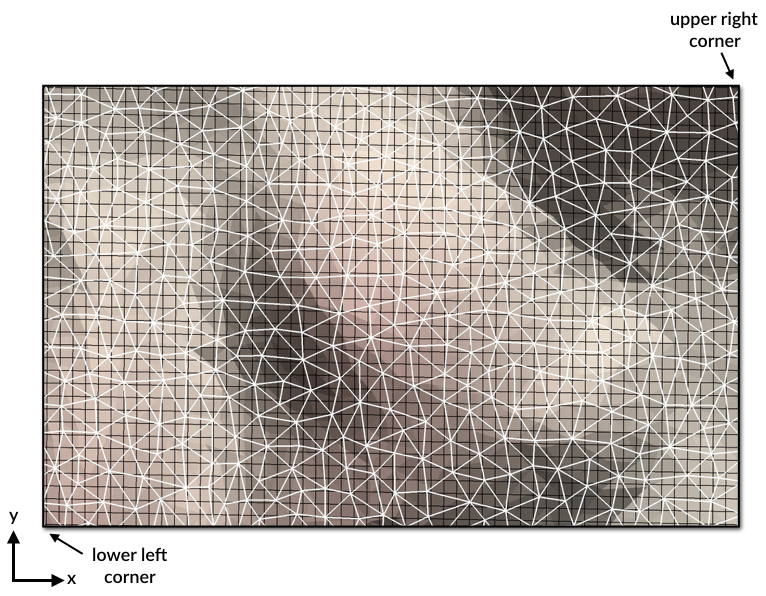
pyBadlands main calculations are performed on a triangular irregular network (TIN). However the code creates its own triangulation based on regularly defined dataset.
Tip
In that way, the user is only required to provide some simple regularly spaced dataset. A similar approach is used for any other maps (e.g. rain, tectonics…).
The only requirement is to follow a specific order for the declaration of each nodes values. To create a simple surface or extract a surface from eTopo grid, you can follow the examples provided in the Companion (simple geometrical model and etopo1).
The order starts from the lower left corner to the upper right corner based on a row-wise indexing (along the X-axis first) as shown in the figure below:
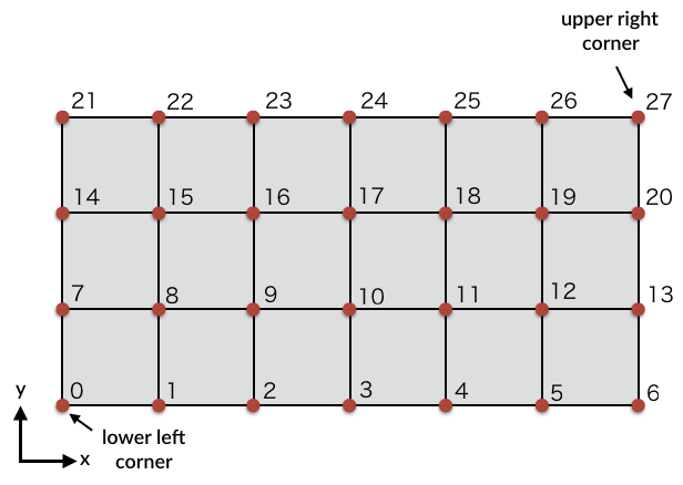
From the regular grid, the TIN is then created within badlands with a resolution which is at maximum equal to the regular grid resolution provided by the user but which could be coarsened if the <resfactor> is set above one in the grid structure.
Time structure
The time structure is also a required element in the XML input and defines the duration of the simulation from start to end time (in years). It is worth noting that these times can be negative, for example <start> can be equal to -150,000 years and <end> to -75,000 years. The only requirement is that start time needs to be lower than end time… (don’t forget this is a forward model!)
In cases where a model is restarted from a previous run, the <restart> element can be used and requires the previous model output folder and the step at which the new simulation needs to restart.
Caution
If the simulation is not restarting this element needs to be commented or deleted.
By default when using the conventional stream power law incision, the code defines its own time step to ensure stability. The user however has the ability to control the minimum and maximum time step allowed.
Lastly, the user needs to define the display interval (<display>) that corresponds to the time step (in years) when an output is created. Depending of the size of your model, decreasing the number of output by increasing the display interval will make your simulation run quicker. When a stratigraphic mesh is recorded by the model (see next structure) the user can decide to output it not at every display interval but at any specific multiple of it. Again this may help to run a model faster.
<!-- Simulation time structure -->
<time>
    <!-- Restart structure -->
    <restart>
      <!-- Model output folder name to restart the simulation from -->
      <rfolder>output_01</rfolder>
      <!-- Model output file step number to restart the model from -->
      <rstep>3</rstep>
    </restart>
    <!-- Simulation start time [a] -->
    <start>0.</start>
    <!-- Simulation end time [a] -->
    <end>100000.</end>
    <!-- Minimum time step [a]. Default is 1. -->
    <mindt>1.</mindt>
    <!-- Maximum time step [a] (optional).
         Set to display interval is not provided. -->
    <maxdt>1000.</maxdt>
    <!-- Display interval [a] -->
    <display>5000.</display>
    <!-- Mesh output frequency based on the display interval. (integer)
         Considering a display interval of T yrs and a mesh output of K
         the mesh will be stored every T*K yrs - (optional default is 1) -->
    <meshout>28</meshout>
</time>
Stratal structure
This element is optional and needs to be loaded in cases where you want to record the stratigraphic architecture over time. It requires 2 parameters. First the horizontal resolution of the mesh that will be used to record the deposition thicknesses over time. This grid can have as a maximum the resolution of the topographic grid or can have a coarser resolution that needs to be a factor of the topographic grid resolution.
<!-- Simulation stratigraphic structure -->
<strata>
    <!-- Stratal grid resolution [m] -->
    <stratdx>500.</stratdx>
    <!-- Stratal layer interval [a] -->
    <laytime>2500.</laytime>
    <!-- Surface porosity  -->
    <poro0>0.52</poro0>
    <!-- characteristic constant for Athy's porosity law  [/km] -->
    <poroC>0.47</poroC>
</strata>
The second parameter is the time interval used to record the stratigraphic grid (<laytime>). It could be the same as the display interval or a smaller interval as long as it remains a multiple of it. For example, if your display interval is set to 25,000 <laytime> can for example be 25,000 or 12,500 or 5,000…
All clastic sediments are subject to compaction (and reduction of porosity) as the result of increasingly tighter packing of grains under a thickening overburden. Porosity decreases with depth, initially largely due to mechanical compaction of the sediment. The decrease in porosity is relatively large close to the seafloor, where sediment is loosely packed; the lower the porosity, the less room there is for further compaction. This decrease in porosity with depth is commonly modelled as a negative exponential function (Athy, 1930). This is an empirical equation, as there is no direct physical link between depth and porosity; compaction and porosity reduction are more directly related to the increase in effective stress under a thicker overburden. Here we only address the simplest scenario with no overpressured zones.
For normally pressured sediments, Athy’s porosity-depth relationship can be expressed in the form:
where the porosity \(\phi\) varies with depth (\(d\)) based on surface porosity \(\phi_0\) defined in the XmL by the element (<poro0>) and \(c\) a coefficient with the units [\(km^{−1}\)] (<poroC>).
Note
Athy, L.F. (1930): Density, Porosity and Compaction of Sedimentary Rocks. Bulletin of the American Association of Petroleum Geologists (AAPG Bulletin), 14, 1-24.
Sea-level structure
By default, the sea-level position in badlands is set to 0 m. If you wish to set it to another position you can use the <position> parameter that changes the sea-level to a new value relative to sea-level. Another option consists in defining your own sea-level curve (<curve>) or using a published one (e.g. Haq curve for example). To create your own sea-level curve, one can use the following example from the Companion toolSea class.
<!-- Sea-level structure -->
<sea>
    <!-- Relative sea-level position [m] -->
    <position>-100.</position>
    <!-- Sea-level curve - (optional) -->
    <!--curve>data/sealvl.csv</curve-->
</sea>
Important
The sea-level curve is defined as a 2 columns ASCII file containing in the first column the time in years (they don’t need to be regularly temporally spaced) and in the second the sea-level position for the given time. When the model runs, it will interpolate linearly between the defined times to define the position of the sea-level.
Tectonic structure
<!-- Tectonic structure -->
<tectonic>
    <!-- Is 3D displacements on ? (1:on - 0:off). Default is 0.-->
    <disp3d>0</disp3d>
    <!-- Only relevant when 3D displacements is on.
         Closest distance [m] between nodes before
         merging happens. This is optional if not given
         the merging distance is set to half the resolution
         of the digital elevation input file. -->
    <merge3d>200.</merge3d>
    <!-- Only relevant when 3D displacements is required.
         This is useful if the horizontal displacements provided
         in each maps are larger than the TIN resolution. In this
         case, it is recommended to split each displacement periods
         in evenly spaced intervals of given time duration [a]. -->
    <time3d>5000.</time3d>
    <!-- Number of tectonic events -->
    <events>1</events>
    <!-- Displacement definition -->
    <disp>
        <!-- Displacement start time [a] -->
        <dstart>5.</dstart>
        <!-- Displacement end time [a] -->
        <dend>10.0</dend>
        <!-- Displacement map [m] -->
        <dfile>data/disp1D.csv</dfile>
    </disp>
</tectonic>
As for the sea-level structure, the tectonic one is optional. Badlands accepts both horizontal and vertical displacements.
Note
These displacements are either lithospheric or mantle induced but the code does not care about what is inducing these changes.
Nevertheless the definition of both vertical-only and horizontal+vertical displacements requires the declaration of different parameters.
In the most simple case of vertical-only displacements (i.e. uplift or subsidence) the model requires:
- the declaration of the element
<events>that basically defines the number of tectonic fields to be applied during the simulation duration, - the definition of each displacement event
<disp>.
Caution
You will need to make sure that the number of events matches the number of displacements defined.
Each displacement requires a start (<dstart>) and end (<dend>) time and a displacement map (<dfile>). The displacements map in the vertical-only case if defined as a ASCII file containing 1 column ordered in the same way as the topography file (lower left corner to upper right one based on row-wise indexing). The values of each node is set based on the desired displacement field and corresponds to the cumulative displacements during the given period.
The second, more complex, option (<disp3d> set to 1; i.e. horizontal+vertical displacements) requires additional parameters.
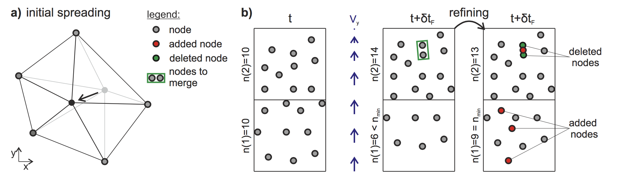
Due to tectonic advection, the density of the surface nodes evolves over time, which leads to areas showing rarefaction or accumulation of nodes. In order for the interpolation schemes to remain accurate and to avoid unnecessary computations, a local addition and deletion of nodes and the consequent remeshing of the triangulated surface are therefore required. This is done by defining the closest distance between nodes before merging happens (<merge3d>). The addition of points is done automatically based on the resolution of the initial topographic grid. To avoid unnecessary remeshing and prevents a huge distortion of the grid due to advection, user is required to set an internal time step for remeshing (<time3d>).
Finally, the definition of the displacement file (<dstart>), in this case, requires the declaration of the cumulative displacements over the given period along the X, Y and Z directions. Thus this file has 3 columns (for each coordinates) and follows the same order as the topographic file. For an in-depth understanding of the technique, users need to look at the 3D surface deformations proposed by Thieulot et al., 2014.
Note
- Thieulot, P. Steer, and R. S. Huismans - Three-dimensional numerical simulations of crustal systems undergoing orogeny and subjected to surface processes, Geochemistry, Geophysics, Geosystems, vol. 15, no. 12, pp. 4936–4957, 2014.
Precipitation structure
Except in cases where you are only interested in aerial evolution associated to hillslope processes only, you will need to define the precipitation structure to account for fluvial related sediment transport.
Like for the tectonic structure, you will be able to define both spatial and temporal changes in the precipitation regime over the simulation time. The first element (<climates>) specifies the number of temporal rain event that you will impose. You will need to ensure that this number matches with the number of (<rain>) element that will be declared (otherwise the code will complain during execution).
<!-- Precipitation structure
     The following methods can be used:
        - an uniform precipitation value for the entire region [m/a]
        - a map containing precipitation values for each nodes of the regular grid
        - a linear elevation dependent precipitation function
        - an orographic precipitation computed using Smith & Barstad theory (2004)
-->
<precipitation>
    <!-- Number of precipitation events -->
    <climates>4</climates>
    <!-- Uniform precipitation definition -->
    <rain>
        <!-- Rain start time [a] -->
        <rstart>0.</rstart>
        <!-- Rain end time [a] -->
        <rend>100000.</rend>
        <!-- Precipitation value [m/a] -->
        <rval>1.</rval>
    </rain>
    <!-- Precipitation map definition -->
    <rain>
        <!-- Rain start time [a] -->
        <rstart>100000.</rstart>
        <!-- Rain end time [a] -->
        <rend>200000.</rend>
        <!-- Precipitation map [m/a] -->
        <map>data/rainLR.csv</map>
    </rain>
The <rain> structure contains at least 3 parameters: the start and end time of the given event and the definition of the precipitation values in metres per year. For this last parameter, three methods are available:
- an uniform precipitation value for the entire region (
<rval>), - a precipitation map containing spatially varying values (
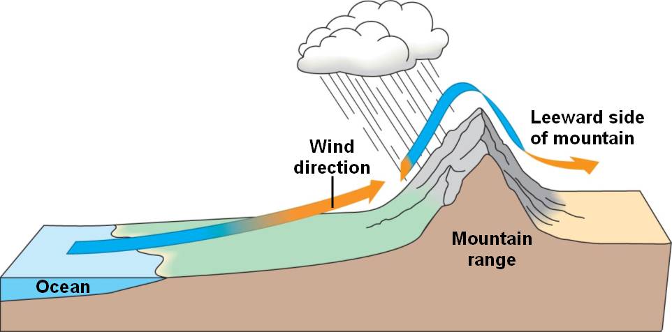
<map>), again this map is defined as a ASCII file containing 1 column ordered in the same way as the topography file (lower left corner to upper right one based on row-wise indexing), - an orographic precipitation model which accounts for the change in rainfall patterns associated to change in topography. The orographic precipitation uses Smith & Barstad (2004) linear model to compute topographic induced rain field and potential values are provided in the example below.
Note
Smith R.B. and Barstad I. : A linear theory of orographic precipitation, Journal of the Atmospheric Sciences, vol. 61, no. 12, pp. 1377–1391, 2004.
    <!-- Linear orographic precipitation model definition -->
    <rain>
      <!-- Rain start time [a] -->
      <rstart>200000.</rstart>
      <!-- Rain end time [a] -->
      <rend>300000.</rend>
      <!-- Rain computation time step [a] -->
      <ortime>5000.</ortime>
      <!-- Minimal precipitation value [m/a] -->
      <rmin>0.2</rmin>
      <!-- Maximal precipitation value [m/a] -->
      <rmax>5.</rmax>
      <!-- Maximal elevation for computing linear trend [m] -->
      <rzmax>3000.</rzmax>
    </rain>
    <!-- Orographic precipitation model definition -->
    <rain>
        <!-- Rain start time [a] -->
        <rstart>300000.</rstart>
        <!-- Rain end time [a] -->
        <rend>400000.</rend>
        <!-- Rain computation time step [a] -->
        <ortime>5000.</ortime>
        <!-- Background precipitation value [m/a] -->
        <rbgd>1.</rbgd>
        <!-- Minimal precipitation value [m/a] -->
        <rmin>0.2</rmin>
        <!-- Maximal precipitation value [m/a] -->
        <rmax>4.</rmax>
        <!-- Wind velocity along X (W-E) direction [m/s] -->
        <windx>-3.</windx>
        <!-- Wind velocity along Y (S-N) direction [m/s] -->
        <windy>2.</windy>
        <!-- Time conversion from cloud water to hydrometeors
             range from 200 to 2000 [s]. Optional default is set
             to 1000 s -->
        <tauc>1000.</tauc>
        <!-- Time for hydrometeor fallout range from 200 to 2000 [s].
             Optional default is set to 1000 s -->
        <tauf>1000.</tauf>
        <!-- Moist stability frequency range from 0 to 0.01 [/s].
             Optional default is set to 0.005 /s -->
        <nm>0.005</nm>
        <!-- Uplift sensitivity factor range from 0.001 to 0.02 [kg/m3].
             Optional default is set to 0.005 kg/m3 -->
        <cw>0.005</cw>
        <!-- Depth of the moist layer range from 1000 to 5000 [m].
             Optional default is set to 3000 m -->
        <hw>3000.</hw>
    </rain>
</precipitation>
Surface processes structure
Several formulations of river incision have been implemented and describe different erosional behaviours ranging from detachment limited, governed by bed resistance to erosion, to transport limited, governed by flow capacity to transport sediment available on the bed.
The default law available in badlands is based on the detachment-limited equation, where erosion rate \(\dot{\epsilon}\) depends on drainage area \(A\), net precipitation \(P\) and local slope \(S\) and takes the form:
\(\kappa_{d}\) (defined as the <erodibility> element in the XmL) is a dimensional coefficient describing the erodibility of the channel bed as a function of rock strength, bed roughness and climate, \(l\), \(m\) and \(n\) are dimensionless positive constants and are set using <m> and <n> respectively. Default formulation assumes \(l = 0\), \(m = 0.5\) and \(n = 1\).
This law is often used to look at purely erosive model (<dep>=0), but as our goal is to not only look at erosion but also at the evolution of sedimentary basin, we need to set additional parameters.
<!-- Stream power law parameters:
The stream power law is a simplified form of the usual expression of
sediment transport by water flow, in which the transport rate is assumed
to be equal to the local carrying capacity, which is itself a function of
boundary shear stress. -->
<sp_law>
<!-- Make the distinction between purely erosive models (0) and erosion /
deposition ones (1). Default value is 1. -->
<dep>1</dep>
<!-- Critical slope used to force aerial deposition for alluvial plain,
in [m/m] (optional). -->
<slp_cr>0.001</slp_cr>
<!-- Maximum percentage of deposition at any given time interval from rivers
sedimentary load in alluvial plain. Value ranges between [0,1] (optional). -->
<perc_dep>0.5</perc_dep>
<!-- Maximum lake water filling thickness. This parameter is used
to defined maximum water level in depression area.
Default value is set to 200 m. -->
<fillmax>50.</fillmax>
<!-- Values of m and n indicate how the incision rate scales
with bed shear stress for constant value of sediment flux
and sediment transport capacity.
Generally, m and n are both positive, and their ratio
(m/n) is considered to be close to 0.5 -->
<m>0.5</m>
<n>1.0</n>
<!-- The erodibility coefficient is scale-dependent and its value depends
on lithology and mean precipitation rate, channel width, flood
frequency, channel hydraulics. In case where the erodibility
structure is turned on, this coefficient is applied to the reworked
sediments. -->
<erodibility>1.e-6</erodibility>
<!-- Number of steps used to distribute marine deposit.
Default value is 5 (integer). (optional)-->
<diffnb>5</diffnb>
<!-- Proportion of marine sediment deposited on downstream nodes. It needs
to be set between ]0,1[. Default value is 0.9 (optional). -->
<diffprop>0.2</diffprop>
<!-- Scaling parameter for diffprop (it depends on the diffprop parameter) value that is dependent on local
topographic slope. Recommended value is 2000.0. Comment out or remove
to revert to fixed diffprop value for entire domain. See Thran et
al. 2020, G-cubed in which diffprop is set to 1.-->
<propa>2000.</propa>
<!-- Additional necessary scaling parameter for slope-dependent diffprop (subject to diffprop parameter value).
Recommended value is 0.005. Comment out or remove to revert to fixed
diffprop value for entire domain. -->
<propb>0.005</propb>
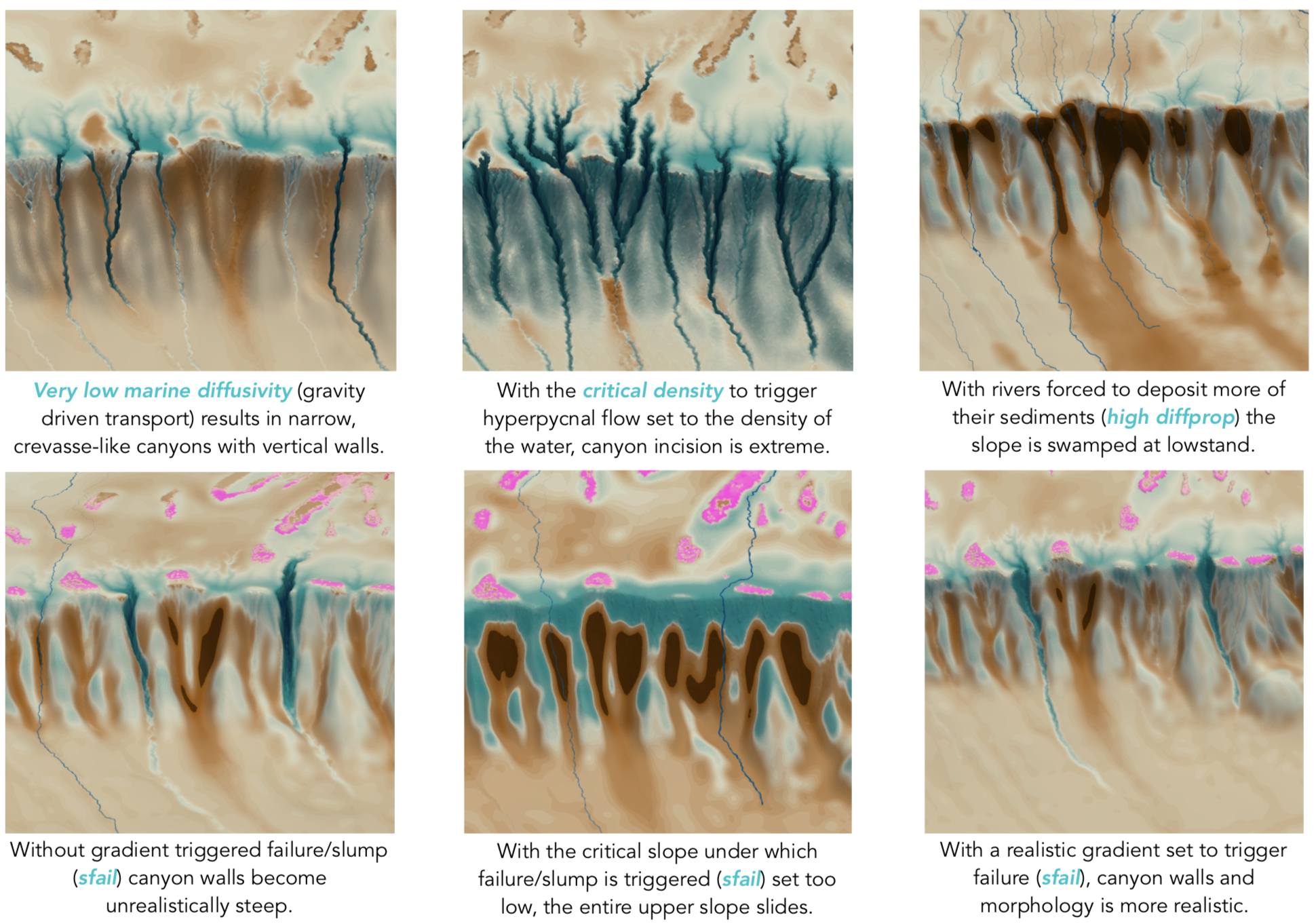
<!-- Critical density of water+sediment flux to trigger hyperpycnal current
off shore - (optional) -->
<dens_cr>1060.</dens_cr>
<!-- Deep basin depth under which hyperpycnal flow are forced to
deposit [m] - (optional) -->
<deepbasin>-2500.</deepbasin>
</sp_law>
Depression – pit sedimentation
The first place where deposition will occur is in depression area. The code will first look for these regions and will estimate the volume of sediment required to fill the depression with a pit-filling algorithm.
Then based on the available amount of sediment transported by the rivers to the depression and the value of the parameter <fillmax>, the filling will start. The parameter <fillmax> corresponds to the maximum elevation (in metres) of a potential lake that forms during one time step in badlands.
Warning
Decreasing the elevation of the lake will increase the number of iteration required to fill the depression, potentially increasing the resolution of the stratigraphic layers but in the same time increasing the model run time…
Alluvial plain forced deposition
The advantage of the detachment law, over the transport-limited approaches, is in the small restriction on computational time steps.
The problem however, is that this detachment law is more suitable for mountainous regions and can not account for alluvial plain deposits.
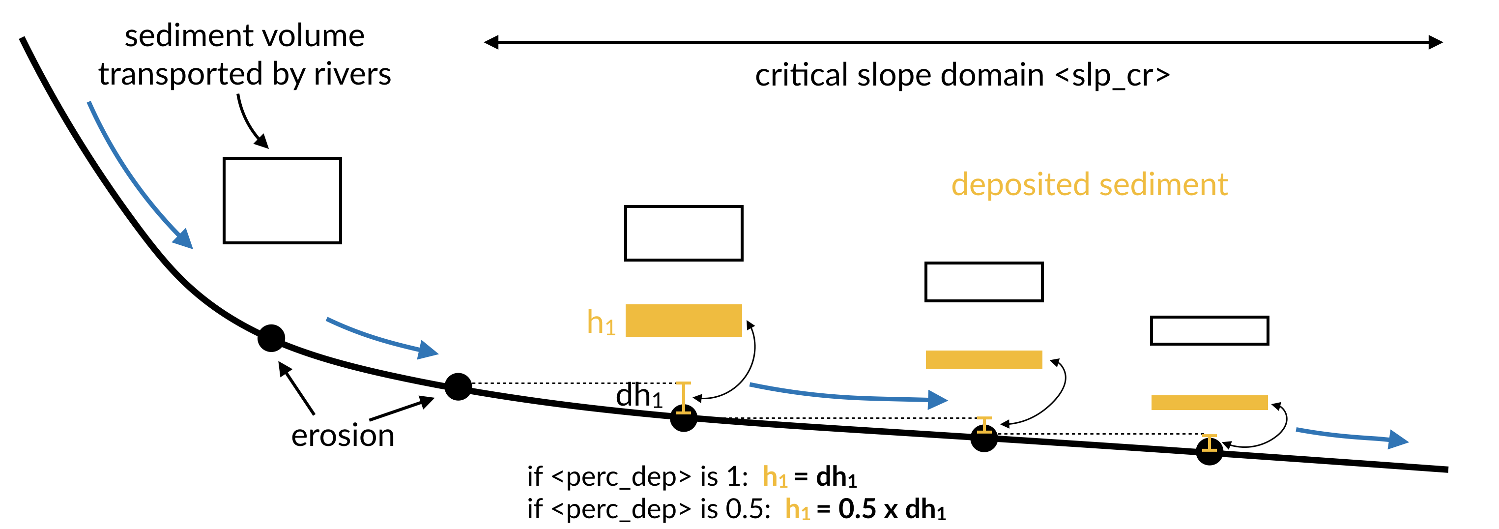
To simulate these deposits in badlands, one can force the deposition when river beds reach a critical slope (<slp_cr>) and the amount of deposition is limited to a percentage of the maximum deposition that ensure no slope reversal (<perc_dep>).
Marine deposition
Once the sediment reaches the marine environment, rivers stop transporting them and sediment are usually deposited close to the shoreline.
Important
A diffusion law, defined within the hillslope structure, allows to diffuse marine sediments.
In addition to the diffusive transport, one can choose to transport the sediment further in the marine realm based on sediment delivery to coasts and marine slopes. To do so you will have to define two additional parameters (<diffnb> and <diffprop>).
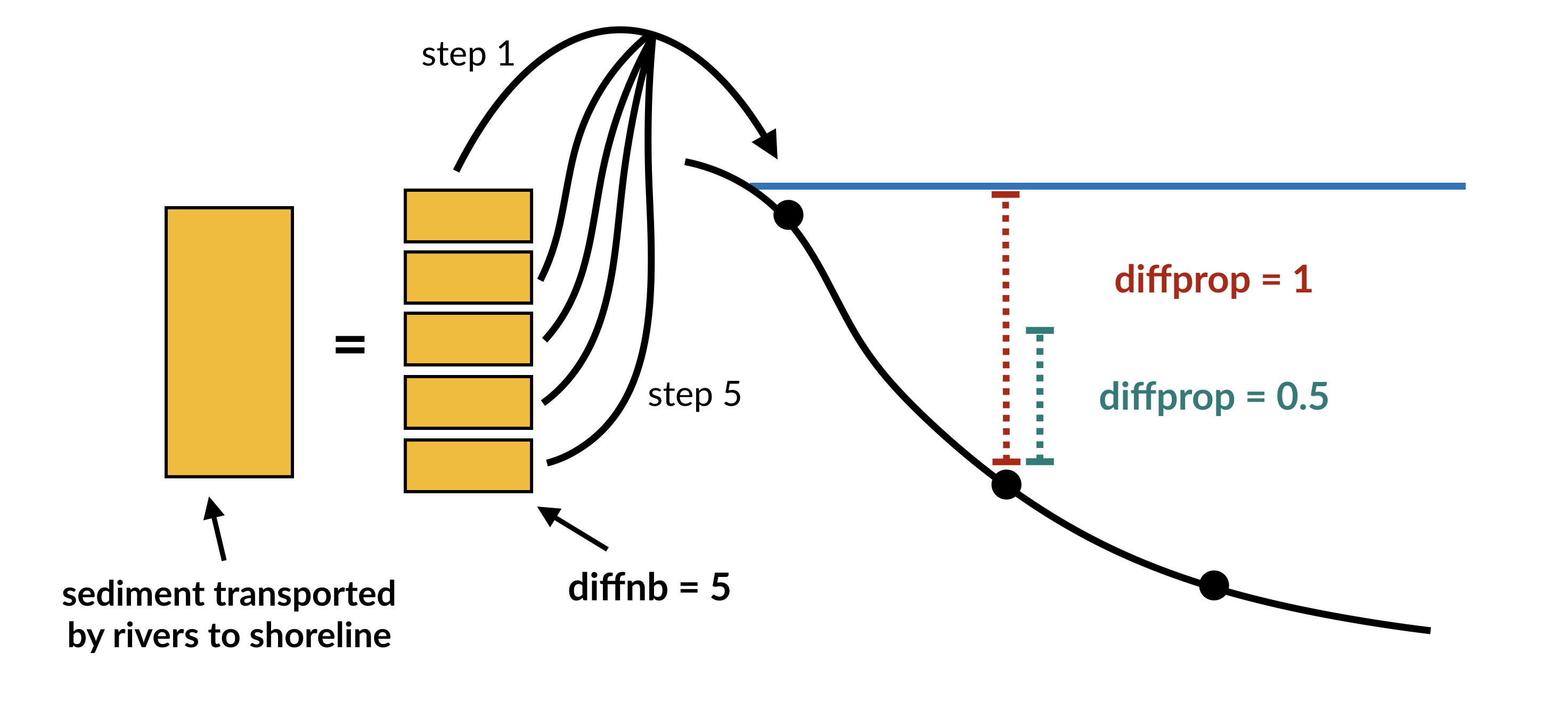
<diffnb> is used to divide the initial volume in several equal parts that will be distributed iteratively over the model time step. <diffprop> relates to a proportion of the maximum thickness that can be deposited on a given nodes based on surrounding elevations.
Marine erosion
In cases where hyperpycnal flows needs to be modelled the user needs to specify the critical density of water and sediment flux required to trigger these currents offshore. It enables to simulate submarine erosion and is set using the <dens_crit> parameter. To be enable <deepbasin> parameter will also need to be set and represent the depth under which hyperpycnal flows will be forced to deposit.
Transport-limited processes
In cases where the flow capacity to erode sediments needs to be taken into account, one needs to specify additional coefficients in the XmL input file.
For a list of available transport-limited laws the user can refer to the simulated processes section on fluvial processes.
The volumetric sediment transport capacity (\(Q_t\)) is defined using a power law function of unit stream power:
where \(\kappa_{t}\) is a dimensional coefficient describing the transportability of channel sediment and \(m_t\) and \(n_t\) are dimensionless positive constants.
A list of 4 different laws are available and summarised in the graph given in the simulated processes section. They are set using the <modeltype> element:
- 0 – detachment limited,
- 1 – undercapacity model (pure cover),
- 2 – tool & cover (almost parabolic),
- 3 – tool & cover (Turowski model), and
- 4 – saltation abrasion.
<!-- Flux-dependent function structure  (optional)
     It is possible to modify the general detachment limited law to simulate channel
     evolution governed by sediment flux–dependent bedrock incision rules.
     Visit tinyurl.com/badlands-incision for more information.
-->
<sedfluxfunction>
    <!-- Incision model type is defined with an integer between 0 and 4:
          + 0 - detachment limited (default) does not required to set additional parameters.
          + 1 - generalised undercapacity model (linear sedflux dependency) [cover effect]
          + 2 - parabolic sedflux dependency [tool & cover effect]
          + 3 - Turowski sedflux dependency [tool & cover effect]
          + 4 - saltation abrasion incision model
         See Hobley et al. (2011), JGR, 116 for more information.
    -->
    <modeltype>0</modeltype>
    <!-- Volumetric sediment transport capacity formulation is built with a stream power law
         and requires the definition of 2 exponents for water discharge (mt) and slope (nt). -->
    <mt>1.5</mt>
    <nt>1.</nt>
    <!-- Transportability of channel sediment (erodibility coefficient) -->
    <kt>2.e-6</kt>
    <!-- Power law relation between channel width and discharge -->
    <kw>1</kw>
    <b>0.5</b>
    <!-- Erodibility dependence to the precipitation is defined with an exponent.
       Default value is set to 0. See Murphy et al. (2016), Nature, 532. -->
    <mp>0.</mp>
    <!-- Bedload versus slope dependency. This option changes the amount of incision based on
         the proportion of bedload material (i.e. gravels) present in stream. For any point in
         the landscape the amount of bedload material is assumed slope-dependent. The user can
         choose between the following options:
          + 0 - no dependency (default)
          + 1 - linear dependency
          + 2 - exponential growth
          + 3 - logarithmic growth
    -->
    <bedslp>0</bedslp>
</sedfluxfunction>
The only remaining parameter defined in the sedfluxfunction structure that can be used with the detachment limited model is the parameter <mp> corresponding to the coefficient l in the SPL law. All the other parameters correspond to the erodibility and coefficients values found in the transport-limited incision formulations.
Note
It is worth noting that the values for the erodibilities vary quite substantially between the different laws (see table below) as well as for the exponent values.
Important
Also in the case of transport-limited simulation, the maximum time step <maxdt> defined in the time structure needs to be reduced to avoid numerical instabilities.
| Parameters | Value |
|---|---|
| \(m_t\) | 1.5 |
| \(n_t\) | 1 |
| \(\kappa_t\) – \(m^{3-2m_t}/yr\) | 2 x \(10^{-5}\) |
| \(\kappa_{SP}\) – \(m^{-(2m+1)}/yr\) | 4 x \(10^{-5}\) |
| \(\kappa_{SA}\) – \(m^{-0.5}\) | 5 x \(10^{-2}\) |
| \(\kappa_{GA}\) – \(m^{-1}\) | 7 x \(10^{-3}\) |
| \(m\) | 0.5 for detach., -0.25 for saltation-abrasion, 0 for abrasion-incision |
| \(n\) | 1 for detach., -0.5 for saltation-abrasion, 0 for abrasion-incision |
| \(\kappa_w\) – \(m^{1-3b}/yr^b\) | 1 |
| \(b\) | 0.5 |
Erodibility structure
The erodibility structure <erocoeff> allows to define a number of initial erodibility layers of varying spatial values. First one needs to define the number of layers to set for the simulation (<erolayers>).
<!-- Erodibility structure simple
     This option allows you to specify different erodibility values either on the surface
    or within a number of initial stratigraphic layers. -->
<erocoeff>
    <!-- Number of erosion layers. -->
    <erolayers>4</erolayers>
    <!-- The layering is defined from top to bottom, with:
        - either a constant erodibility value for the entire layer or with an erodibility map
        - either a constant thickness for the entire layer or with a thickness map -->
    <!-- Constant erodibility and layer thickness -->
    <erolay>
        <!-- Uniform erodibility value for the considered layer. -->
        <erocst>3.e-6</erocst>
        <!-- Uniform thickness value for the considered layer [m]. -->
        <thcst>10</thcst>
    </erolay>
    <!-- Constant erodibility and variable layer thickness map -->
    <erolay>
        <!-- Uniform erodibility value for the considered layer. -->
        <erocst>3.e-6</erocst>
        <!-- Variable thicknesses for the considered layer [m]. -->
        <thmap>data/thlay2.csv</thmap>
    </erolay>
    <!-- Variable erodibilities and constant layer thickness -->
    <erolay>
        <!-- Variable erodibilities for the considered layer. -->
        <eromap>data/erolay3.csv</eromap>
        <!-- Uniform thickness value for the considered layer [m]. -->
        <thcst>30</thcst>
    </erolay>
    <!-- Variable erodibilities and thicknesses -->
    <erolay>
        <!-- Variable erodibilities for the considered layer. -->
        <eromap>data/erolay4.csv</eromap>
        <!-- Variable thicknesses for the considered layer [m]. -->
        <thmap>data/thlay4.csv</thmap>
    </erolay>
</erocoeff>
Each layer can be either of uniform erodibility values (<erocst>) or defined as a multi-erodibility map (<eromap>).
<!-- Erodibility structure with multiple rock types
     This option allows you to specify different erodibility values based on different
     rock types. The approach tracks rocks erosion/transport/deposition through space and
     time over the simulated domain.
     NOTE:
     In this first version, the algorithm is not working with 3D displacements for now and
     is pretty slow.-->
<erocoeffs>
    <!-- Active layer thickness [m]-->
    <actlay>1.</actlay>
    <!-- Number of rock types to track. -->
    <rocktype>4</rocktype>
    <!-- Stratal layer interval [a] -->
    <laytime>2500.</laytime>
    <!-- Definition of erodibility values for each rock types -->
    <rockero>
        <!-- Erodibility coefficient for rock type 1 -->
        <erorock>5.e-6</erorock>
    </rockero>
    <rockero>
        <!-- Erodibility coefficient for rock type 2 -->
        <erorock>8.e-9</erorock>
    </rockero>
    <rockero>
        <!-- Erodibility coefficient for rock type 3 -->
        <erorock>2.e-6</erorock>
    </rockero>
    <rockero>
        <!-- Erodibility coefficient for rock type 4 -->
        <erorock>4.e-6</erorock>
    </rockero>

    <!-- Number of erosion layers. -->
    <erolayers>4</erolayers>
    <!-- The layering is defined from top to bottom, with a file containing the
         following properties for each points of the regular grid (DEM):
          - 1st column the thickness of the considered layer
          - 2nd column the rock type ID (an integer) -->
    <!-- Constant erodibility and layer thickness -->
    <erolay>
        <!-- Uniform erodibility value for the considered layer. -->
        <laymap>data/thlaytop.csv</laymap>
    </erolay>
    <erolay>
        <!-- Uniform erodibility value for the considered layer. -->
        <laymap>data/thlay2.csv</laymap>
    </erolay>
    <erolay>
        <!-- Uniform erodibility value for the considered layer. -->
        <laymap>data/thlay3.csv</laymap>
    </erolay>
    <erolay>
        <!-- Uniform erodibility value for the considered layer. -->
        <laymap>data/thlay4.csv</laymap>
    </erolay>
</erocoeffs>
The definition also requires a thickness for each of these layers that can either be spatially constant (<thcst>) or variable (<thmap>).
Using a combination, one can produced a complex stack of spatially varying subsurface layers. The requirements for any of these maps are the same as for any other badlands grids, i.e. ordered from the lower left corner to the upper right corner based on row-wise indexing (along the X-axis first).
Hillslope structure
Note
Transport along slope by gravity is simulated using 2 types of diffusion laws.
In the first one, you can use a linear law commonly referred to as soil creep:
in which \(\kappa_{hl}\) is the diffusion coefficient and can be set for the marine (<cmarine>) and land (<caerial>) environments.
A second approach, based on a non-linear formulation, assumes that flux rates increase to infinity if slope values approach a critical slope \(S_{c}\):
To use this approach, you will have to define another parameter (<cslp>) corresponding to the critical slope.
<!-- Hillslope diffusion parameters:
     Parameterisation of the sediment transport includes the simple creep transport
     law which states that transport rate depends linearly on topographic gradient. -->
<creep>
    <!-- Surface diffusion coefficient [m2/a] -->
    <caerial>0.001</caerial>
    <!-- Marine diffusion coefficient [m2/a] -->
    <cmarine>0.005</cmarine>
    <!-- Critical slope for non-linear diffusion [m/m] - optional.
         Default value is set to 0 meaning non-lnear diffusion is not considered. -->
    <cslp>0.8</cslp>
    <!-- River transported sediment diffusion
         coefficient in marine realm [m2/a] -->
    <criver>10.</criver>
    <!-- Critical slope above which slope failure are triggered [m/m] - optional.
         Default value is set to 0 meaning non-lnear diffusion is not considered. -->
    <sfail>0.26</sfail>
    <!-- Triggered failure sediment diffusion coefficient [m2/a] -->
    <cfail>3.</cfail>
</creep>
To increase marine transportation of freshly deposited river sediments along the coasts, one can decide to define an additional diffusion coefficient (<criver>) that will promote deep water transport of river-induced marine deposits.
Finally, one can choose to simulate slope failure or slump in aerial and marine environment by defining a critical slope value above which these processes are triggered (<sfail>) and a diffusion coefficient to transport the associated sediments (<cfail>).
Flexural isostasy structure
To estimate flexural isostasy, gflex modular python package is used in badlands. It allows to compute isostatic deflections of Earth’s lithosphere with uniform or non-uniform flexural rigidity and couple the interactions with evolving surface loads induced by erosion/deposition associated to modelled surface processes.
Note
Wickert, A. D. (2016), Open-source modular solutions for flexural isostasy: gFlex v1.0, Geosci. Model Dev., 9(3), 997–1017, doi:10.5194/gmd-9-997-2016.
The flexural isostasy is performed on a regular grid (defined based on the number of nodes along the X and Y axis – <fnx> and <fny>) and user-defined time intervals (<ftime>).
To compute the isostasy additional parameters are required: the mantle density (<dmantle>), the sediment density (<dsediment>), the Young’s Modulus (<youngMod>), the Poisson’s ratio (<poisson>) and the lithospheric elastic thickness.
<!-- Flexural isostasy parameters:
     Parameterisation of the flexural isostasy using the gFlex model from Wickert 2015.
     The current wrapper limits the functionnality of the gFlex algorithm and only uses
     the direct solver of the 2D finite difference method with the van Wees and Cloetingh
     plate solution. -->
<flexure>
    <!-- Time step used to compute the isostatic flexure. -->
    <ftime>10000.0</ftime>
    <!-- Definition of the flexural grid:
         It is possible to setup a flexural grid at a resolution higher than the one used
         for the TIN to increase computational speed. In this case you need to define the
         discretization along X and Y axis. By default the same resolution as the one given
         for the DEM file is used and the following 2 parameters are not required. -->
    <!-- Number of points along the X-axis - (optional)-->
    <fnx>100</fnx>
    <!-- Number of points along the Y-axis - (optional)-->
    <fny>100</fny>
    <!-- Mantle density [kg/m3] -->
    <dmantle>3300</dmantle>
    <!-- Sediment density [kg/m3] -->
    <dsediment>2500</dsediment>
    <!-- Young's Modulus [Pa] -->
    <youngMod>65E9</youngMod>
    <!-- Poisson ratio -->
    <poisson>0.25</poisson>
    <!-- The lithospheric elastic thickness (Te) can be expressed as a scalar if you assume
         a uniform thickness for the model area in this case the value is given in the next
         parameter [m] - (optional) -->
    <elasticH>35000.</elasticH>
    <!-- In case where the lithospheric elastic thickness (Te) varies on the simulated region
         you might want to use a grid defining for each points on the flexural grid the estimate
         Te value [m]. You will need to ensure that the grid dimensions match the number of
         points given for the flexural grid resolution - (optional) -->
    <elasticGrid>data/elasticthickness.csv</elasticGrid>
    <!-- In case where the lithospheric elastic thickness (Te) varies with time.
         The elastic thickness relates to the age of the lithosphere with a simple equation that
         results from the square-root time dependence of lithospheric cooling via thermal conduction.
                        Te = a1 x sqrt(t) + a2
         You will need to define the coefficient for a1 and a2 where a1 is the slope of the dependency
         and a2 the initial elastic thickness [m] at the start of the simulation - (optional) -->
    <elasticA1>2.7</elasticA1>
    <elasticA2>10000.</elasticA2>
Three conditions can be set in regards to the elastic thickness. The simplest one assumes a uniform thickness over the simulated region (<elasticH>). The second defines a spatial variation in elastic thicknesses.
This option requires an input file that needs to be of the same dimension as the flexural grid and needs to follow the conventional badlands ordering approach (from the lower left corner to the upper right corner based on row-wise indexing). The last option considers a time dependent lithospheric elastic thickness Te defined by the following equation:
where \(t\) is the time in years, \(A_1\) and \(A_2\) the coefficients to define in the XmL file.
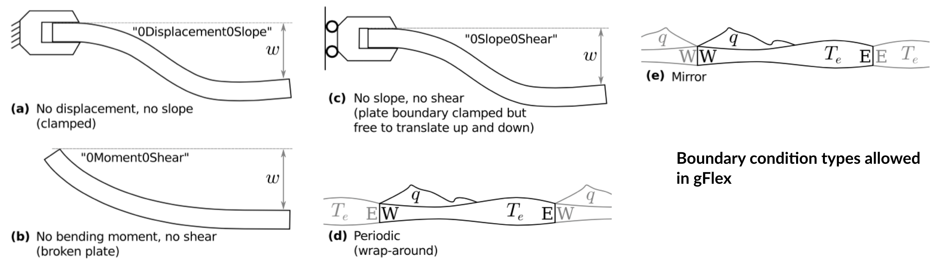
Finally gflex requires the definition of the boundary conditions along each borders (N,S,E,W) and 4 different types are available (as shown in the previous figure).
     <!-- Finite difference boundary conditions:
          + 0Displacement0Slope: 0-displacement-0-slope boundary condition
          + 0Moment0Shear: "Broken plate" boundary condition: second and
                    third derivatives of vertical displacement are 0. This
                    is like the end of a diving board.
          + 0Slope0Shear: First and third derivatives of vertical displacement
                    are zero. While this does not lend itsellf so easily to
                    physical meaning, it is helpful to aid in efforts to make
                    boundary condition effects disappear (i.e. to emulate the
                    NoOutsideLoads cases)
          + Mirror: Load and elastic thickness structures reflected at boundary.
          + Periodic: "Wrap-around" boundary condition: must be applied to both
                    North and South and/or both East and West. This causes, for
                    example, the edge of the eastern and western limits of the domain
                    to act like they are next to each other in an infinite loop.
         The boundary are defined for each edges W, E, S and N. -->
    <boundary_W>0Displacement0Slope</boundary_W>
    <boundary_E>0Displacement0Slope</boundary_E>
    <boundary_S>0Displacement0Slope</boundary_S>
    <boundary_N>0Displacement0Slope</boundary_N>
</flexure>
Wave structure
Wave evolution and associated sediment transport are calculated from a series of equations defined in the model physical description (wave simulation). These equations are solved on a regular grid (resolution: <wres>) and at given time intervals (<twave>).
Important
Impact of wave on sediment transport is limited to shallow areas where water depth is below the wave base value (<wbase>).
The erosion thickness he (<wEro>) is limited to the top sedimentary layers and for simplicity is assumed to follow a logarithmic form:
when \(\tau_w>\tau_c\) where \(C_e\) is an entrainment coefficient (<wCe>) controlling the relationship between shear stress and erosion rate.
Sediment is transported by wave-induced currents over a maximum number of iterations (<tsetps>). Remobilised sediment by wave are then diffused on the grid using a coefficient of diffusion <wCd> and during a number of iterations (<dsteps>).
<!-- Wave global parameters structure -->
<waveglobal>
    <!-- Wave model to consider either SWAN or WaveSed.
         Default is WaveSed (wmodel = 0). -->
    <wmodel>0</wmodel>
    <!-- Wave interval [a] -->
    <twave>250.</twave>
    <!-- Wave grid resolution [m] -->
    <wres>1000.</wres>
    <!-- Maximum depth for wave influence [m] -->
    <wbase>20</wbase>
    <!-- Number of wave climate temporal events. -->
    <events>1</events>
    <!-- Mean grain size diameter [m] -->
    <d50>0.0001</d50>
    <!-- Wave sediment diffusion coefficient. Default is 50. -->
    <wCd>50.</wCd>
    <!-- Wave sediment entrainment coefficient. Value needs to be
         set between ]0,1]. Default is 0.5 -->
    <wCe>0.35</wCe>
    <!-- Maximum wave-induced erosion rate [m/yr] -->
    <wEro>0.002</wEro>
    <!-- Maximum depth for wave influence [m] -->
    <wbase>10</wbase>
    <!--  Steps used to perform sediment transport.
          Default is 1000. -->
    <tsteps>500</tsteps>
    <!--  Steps used to perform sediment diffusion.
          Default is 1000. -->
    <dsteps>500</dsteps>
</waveglobal>
The proposed method consists in producing snapshots of wave-driven circulation distribution resulting from series of deep-water wave scenarios (<climNb>). These wave climates (<climate>) are based on a significant wave height (<hs>), a percentage of activity (<perc>) remaining fixed during the desired time interval (defined in years by <start> and <end> elements) and a mean wave direction (<dir>).
<!-- Wave definition based on wave global structure.
     The wave field needs to be ordered by increasing start time.
     The time needs to be continuous between each field without overlaps. -->
<wave>
    <!-- Wave start time [a] -->
    <start>-14000.</start>
    <!-- Wave end time [a] -->
    <end>0</end>
    <!-- Wave climates number -->
    <climNb>3</climNb>
    <!-- Climatic wave definition for WaveSed model. -->
    <climate>
        <!-- Percentage of time this event is active during the time interval. -->
        <perc>0.3</perc>
        <!-- Significant wave height (in m) -->
        <hs>2.</hs>
        <!-- Wave direction in degrees (between 0 and 360) from the
             X-axis (horizontal) anti-clock wise. It specifies where the waves are
             actually coming from. The wave directions are reduced to 8 possible ones:
             East (dir = 0) - North (dir = 90) - West (dir = 180) - South (dir = 270) -
             NE (0<dir<90) - NW (90<dir<180) - SW (180<dir<270) - SE (dir>270). -->
        <dir>0</dir>
    </climate>
    <!-- Climatic wave definition for WaveSed model. -->
    <climate>
        <!-- Percentage of time this event is active during the time interval. -->
        <perc>0.3</perc>
        <!-- Significant wave height (in m) -->
        <hs>2.</hs>
        <!-- Wave direction in degrees (between 0 and 360) from the
             X-axis (horizontal) anti-clock wise. It specifies where the waves are
             actually coming from. The wave directions are reduced to 8 possible ones:
             East (dir = 0) - North (dir = 90) - West (dir = 180) - South (dir = 270) -
             NE (0<dir<90) - NW (90<dir<180) - SW (180<dir<270) - SE (dir>270). -->
        <dir>30</dir>
    </climate>
    <!-- Climatic wave definition for WaveSed model. -->
    <climate>
        <!-- Percentage of time this event is active during the time interval. -->
        <perc>0.4</perc>
        <!-- Significant wave height (in m) -->
        <hs>2.</hs>
        <!-- Wave direction in degrees (between 0 and 360) from the
             X-axis (horizontal) anti-clock wise. It specifies where the waves are
             actually coming from. The wave directions are reduced to 8 possible ones:
             East (dir = 0) - North (dir = 90) - West (dir = 180) - South (dir = 270) -
             NE (0<dir<90) - NW (90<dir<180) - SW (180<dir<270) - SE (dir>270). -->
        <dir>300</dir>
    </climate>
</wave>
Carbonate structure
Carbonate system evolution in badlands is driven by a set of rules whose variables are fully adjustable (as explained in the carbonate process section).
<!-- Carbonate growth definition based on carbonate global structure.
     The events need to be ordered by increasing start time.
     The time needs to be continuous between each event without overlaps. -->

<carb>
    <!-- Specify initial basement structure (0) for hard rock and (1) for loose sediment. -->
    <baseMap>data/base500south.csv</baseMap>
    <!-- Carbonate growth time interval [a] -->
    <tcarb>50.</tcarb>
    <!-- Specify the number of reef growth events -->
    <growth_events>2</growth_events>
    <!-- Specify Species 1 and 2 growth rates for specific reef growth events-->
    <event>
        <!-- Reef growth event start time [a] -->
        <gstart>-1000.</gstart>
        <!-- Reef growth event end time [a] -->
        <gend>-750.</gend>
        <!-- Species 1 growth rate during event [m/yr]. -->
        <growth_sp1>0.009</growth_sp1>
        <!-- Species 2 growth rate during event [m/yr]. -->
        <growth_sp2>0.005</growth_sp2>
    </event>
    <event>
        <!-- Reef growth event start time [a] -->
        <gstart>-500.</gstart>
        <!-- Reef growth event end time [a] -->
        <gend>-250.</gend>
        <!-- Species 1 growth rate during event [m/yr]. -->
        <growth_sp1>0.</growth_sp1>
        <!-- Species 2 growth rate during event [m/yr]. -->
        <growth_sp2>0.</growth_sp2>
    </event>
</carb>
Two different types of carbonates can be defined (<species1> & <species2>), in addition one can define hemipelagic deposition (<pelagic>).
Important
It is necessary to defined the region where carbonates will preferably grow using a basement map defining loose sediment (1) and hard cover (0). The map here again is a one column ASCII file ordered from the lower left corner to the upper right corner based on row-wise indexing.
<!-- Specify species 1 growth functions based on 3 main controlling forces: depth,
     sedimentation rate and ocean wave height.
     These functions are defined as csv files produced using pre-processing IPython
     notebook. -->

<species1>
    <!-- Depth control on species 1 evolution. -->
    <depthControl>data/depthcontrol1.csv</depthControl>
    <!-- Ocean wave height control on species 1 evolution. -->
    <waveControl>data/wavecontrolcarb1.csv</waveControl>
    <!-- Sedimentation control on species 1 evolution. -->
    <sedControl>data/sedcontrolcarb1.csv</sedControl>
</species1>

<!-- Specify species 2 growth functions based on 3 main controlling forces: depth,
     sedimentation rate and ocean wave height.
     These functions are defined as csv files produced using pre-processing IPython
     notebook. -->
<species2>
    <!-- Species 2 growth rate [m/yr]. -->
    <!-- Depth control on species 2 evolution. -->
    <depthControl>data/depthcontrol2.csv</depthControl>
    <!-- Ocean wave height control on species 2 evolution. -->
    <waveControl>data/wavecontrolcarb2.csv</waveControl>
    <!-- Sedimentation control on species 2 evolution. -->
    <sedControl>data/sedcontrolcarb2.csv</sedControl>
</species2>

<!-- Specify pelagic deposition functions based on depth control.
     The function is defined as csv file produced using pre-processing IPython
     notebook. -->
<pelagic>
    <!-- Pelagic deposition rate [m/yr]. -->
    <growth>0.00005</growth>
    <!-- Depth control on pelagic deposition. -->
    <depthControl>data/pelagiccontrol.csv</depthControl>
</pelagic>
Carbonate evolution is computed at user-defined interval (<tcarb>) and the carbonate production is controlled by a maximum of 3 parameters:
- depth (i.e. accommodation –
<depthControl>), - wave height (
<waveControl>), and - sedimentation rate (
<sedControl>).
These parameters are curves ranging between desired values of depth, sedimentation rate or wave height along the X-axis and [0,1] along the Y-axis. Each species is given a maximum vertical growth rate (<growth>) in metres per year which is then modulated based on the combination of each curve values.
Output structure
The <outfolder> element is optional but is highly recommended as it enables you to specify your ouput folder name. If not specified, the default name will be output.
Important
To prevent the deletion of any output folders if you have not changed the folder name, the code automatically creates a new name which add an underscore and a number at the end of the output filename.
As an example, let us consider you have already ran a model with the <outfolder> element set to ’myexp’ and you have decided to change the erodibility value in the SPL law but kept the folder name the same.
Badlands will create a new folder named ’myexp_0’. If you keep changing any parameters omitting to change the folder name, you will have a list of folders like ’myexp_1’, ’myexp_2’, ’myexp_3’…
    <!-- Output folder path -->
    <outfolder>out</outfolder>

</badlands>