Simulated Processes
Over the last decades, many numerical models have been proposed to simulate how the Earth surface has evolved over geological time scales in response to different driving mechanisms such as tectonics or climatic variability . These models combine empirical data and conceptual methods into a set of mathematical equations that can be used to reconstruct landscape evolution and associated sediment fluxes . They are currently used in many research fields such as hydrology, soil erosion, hillslope stability and general landscape studies.
Numerous models have focused on the erosional processes especially in the case of river dynamics yet much less work has been done to simulate regional to continental depositional systems and associated stratigraphic evolution in sedimentary basins . In addition and with a few exceptions most of these models have either been limited to one part of the sediment routing system (e.g., fluvial geomorphology, coastal erosion, carbonate platform development) or built upon simple laws commonly derived from diffusion-based equations which applications require pluri-kilometric spatial resolution . These limitations often restrict our understanding of sediment fate from source to sink. It also makes it difficult to link site-specific observations to numerical model outputs.
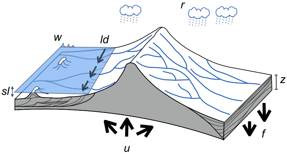
Badlands framework and the development efforts behind it are intended to address these shortcomings. It provides a more direct and flexible description of the inter-connectivities between land, marine and reef environments, in that it explicitly links these systems together (Fig 1). As mentioned above, the focus of badlands is primarily on the description of Earth surface evolution and sedimentary basins formation over regional to continental scale and geological time (thousands to millions of years). Badlands, introduced herein, is view as an integrative framework that provides a simple and adaptable numerical tool to explore Earth surface dynamics and quantify the feedback mechanisms between climate, tectonics, erosion and sedimentation.
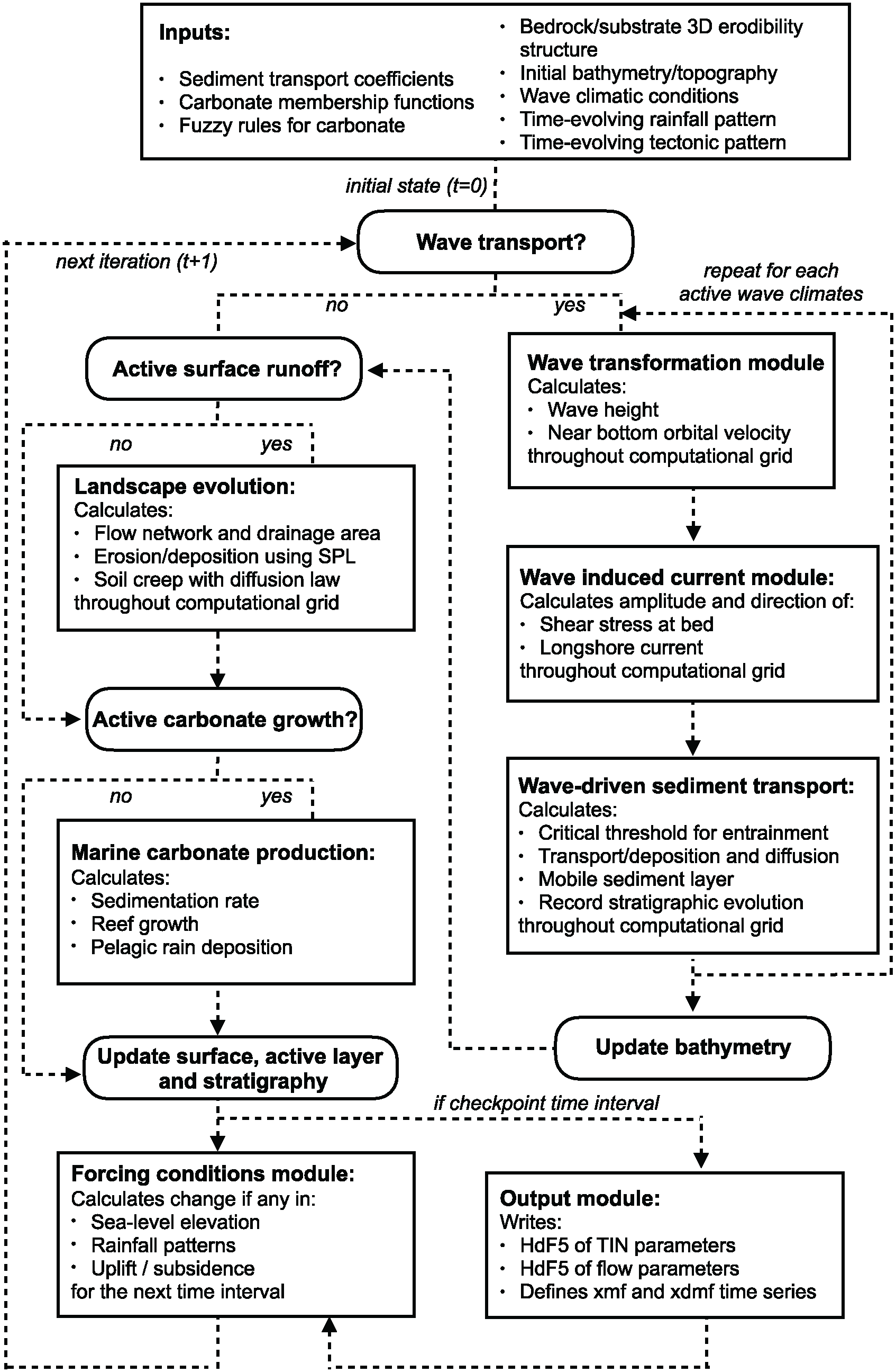
Badlands uses a triangular irregular network (TIN) to solve the geomorphic equations presented below . The continuity equation is defined using a finite volume approach and relies on the method described in Tucker et al. . Fig 2 illustrates the relationships between the different components of the framework.
Fluvial system
To solve channel incision and landscape evolution, the algorithm follows the O(n)-efficient ordering method from Braun and Willett and is based on a single-flow-direction (SFD) approximation assuming that water goes down the path of the steepest slope .
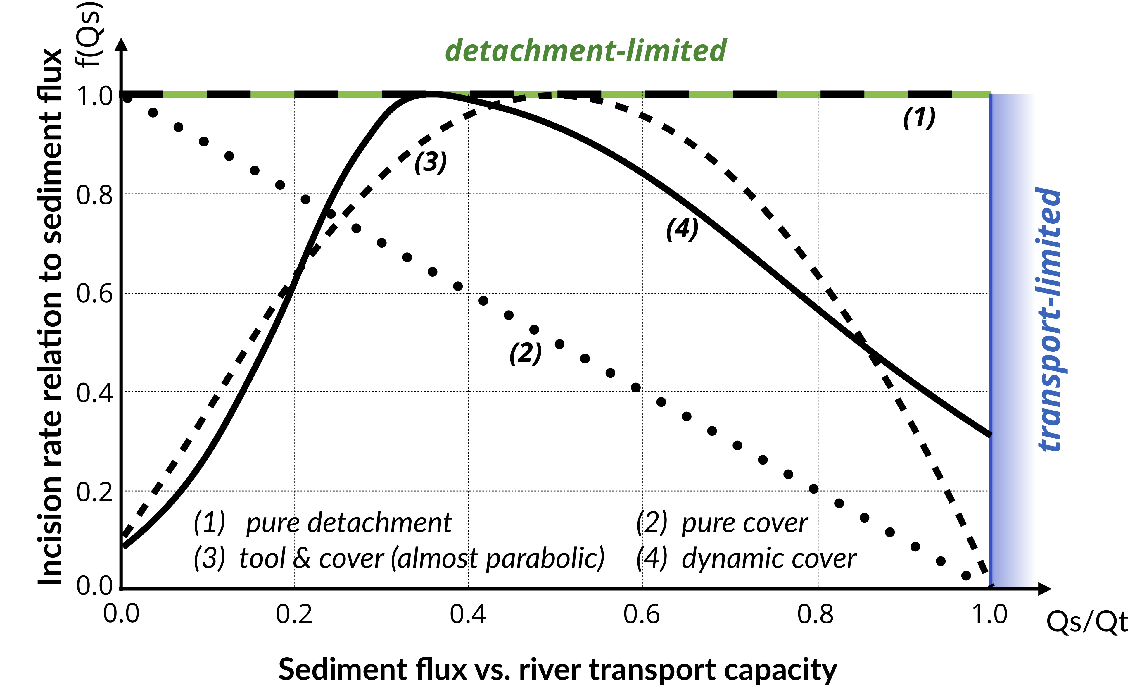
Several formulations of river incision have been proposed to account for long term evolution of fluvial system , . These formulations describe different erosional behaviours ranging from detachment limited, governed by bed resistance to erosion, to transport limited, governed by flow capacity to transport sediment available on the bed. Mathematical representation of erosion process in these formulations is often assumed to follow a stream power law . These relatively simple approaches have two main advantages. First, they have been shown to approximate the first order kinematics of landscape evolution across geologically relevant timescales (\(>{10}^4\) years). Second, neither the details of long term catchment hydrology nor the complexity of sediment mobilisation dynamics are required. Below, we present the six incision laws currently available in badlands (Fig 3).
Detachment-limited model
\[\dot{\epsilon}=\kappa_{d} P^l (PA)^m S^n\]
\(\kappa_{d}\) is a dimensional coefficient describing the erodibility of the channel bed as a function of rock strength, bed roughness and climate, \(l\), \(m\) and \(n\) are dimensionless positive constants. Default formulation assumes \(l = 0\), \(m = 0.5\) and \(n = 1\). The precipitation exponent \(l\) allows for representation of climate-dependent chemical weathering of river bed across non-uniform rainfall .
Transport-limited model
Here, volumetric sediment transport capacity (\(Q_t\)) is defined using a power law function of unit stream power:
\[Q_t=\kappa_{t} (PA)^{m_t} S^{n_t}\]
where \(\kappa_{t}\) is a dimensional coefficient describing the transportability of channel sediment and \(m_t\) and \(n_t\) are dimensionless positive constants. In Eq 2, the threshold of motion (the critical shear stress) is assumed to be negligible .
An additional term is now introduced in the stream power model:
\[\dot{\epsilon}=\kappa f(Q_s) (PA)^m S^n\]
with \(f(Q_{s})\) representing a variety of plausible models for the dependence of river incision rate on sediment flux (Fig 3). In the standard detachment-limited, \(f(Q_{s})\) is equal to unity, which corresponds to cases where \(Q_{s} \ll Q_{t}\). Where sediment flux equals or exceeds transport capacity (\(Q_s/Q_t \ge 1\)) the system is by definition transport-limited (and depositional if \(Q_s/Q_t > 1\)).
This model assumes that stream incision potential decreases linearly from a maximum where there is negligible sediment flux to zero where sediment flux equals transport capacity (Fig 3 - option 2). Conceptually, this law mimics the transfer of stream energy from erosion to transport processes :
\[f(Q_s)=1-\frac{Q_s}{Q_t}\]
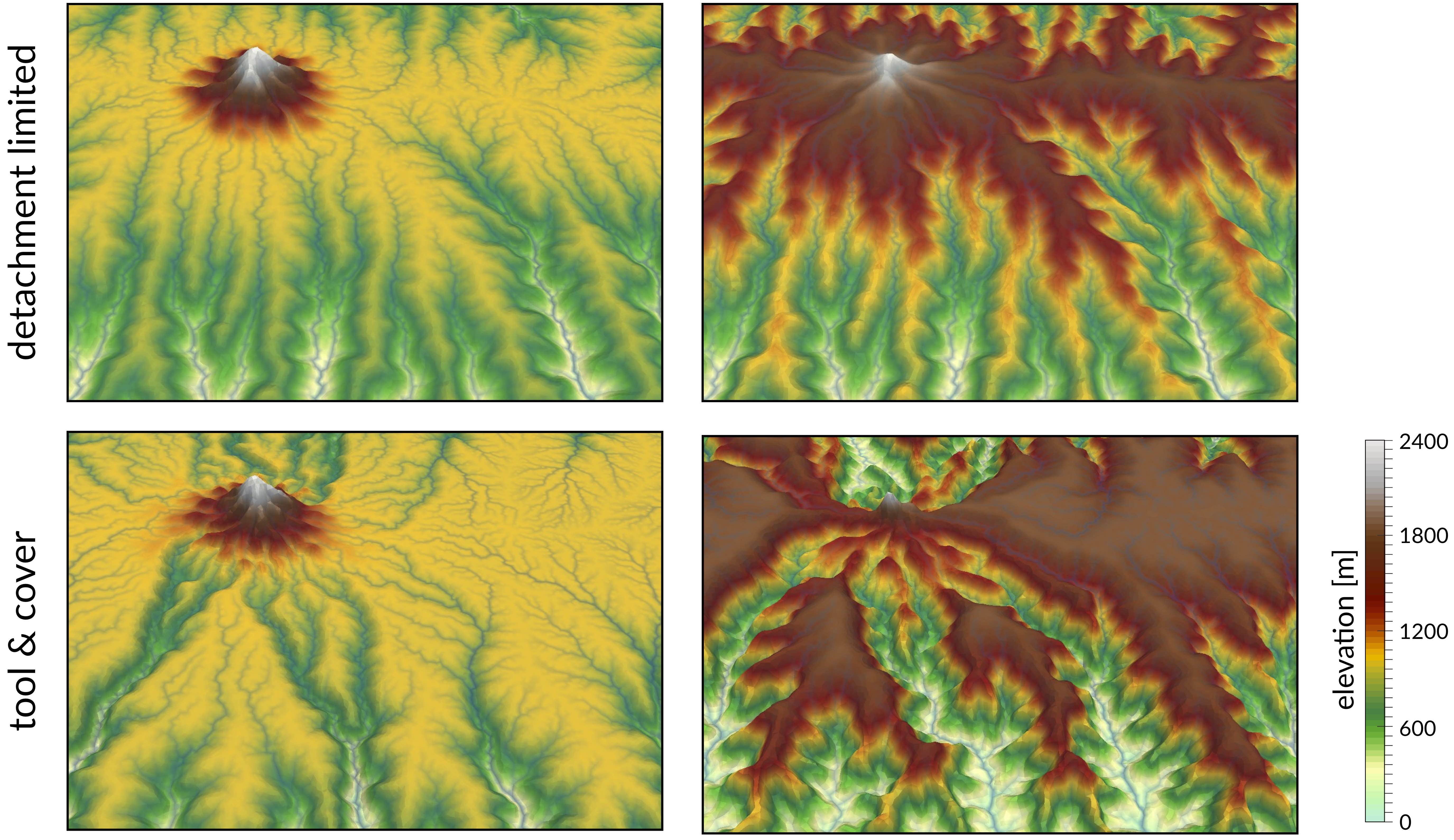
Both qualitative and experimental observations have shown that sediment flux has a dual role in the erosion process. First, when sediment flux is low relative to capacity, erosion potential increases with sediment flux (tool effect: bedrock abrasion and plucking). Then, with increased sediment flux, erosion is inhibited (cover effect: sediments protect the bed from impacts by saltating particles). Following Gasparini et al. , we adopt a parabolic form that reaches a maximum at \(Q_s/Q_t = 1/2\) (Fig 3 - option 3, Fig 4):
\[\begin{split}\begin{eqnarray}
f(Q_s)=1-4\left(\frac{Q_s}{Q_t}-0.5\right)^2 \,\,\,\, \mathrm{if} \,\,\,\, Q_s/Q_t >0.1, \nonumber \\
f(Q_s)=2.6 \frac{Q_s}{Q_t}+0.1 \,\,\,\, \mathrm{if} \,\,\,\, Q_s/Q_t \leq 0.1
\end{eqnarray}\end{split}\]
To account for sediment and spatial heterogeneity of the armouring of the bed, Turowski et al. proposed a modified form of the Almost parabolic model that better estimates the original Sklar and Dietrich experiments (Fig 3 - option 4). It takes the form of two combined Gaussian functions:
\[f(Q_s)=\exp \left[ - \left(\frac{Q_s/Q_t-0.35}{C_h}\right)^2 \right]\]
where \(C_h\) is set to 0.22 for \(Q_s/Q_t \leq 0.35\) and 0.6 when \(Q_s/Q_t > 0.35\).
Sklar & Dietrich proposed also a formulation for tool and cover mechanisms which relates bedrock incision to abrasion of saltating bed load. The expression shares the same form as the sediment flux–dependent incision rule presented by Whipple & Tucker (Eq 3) with significantly different exponent values:
\[\dot{\epsilon}=\kappa_{sa} f(Q_s) A^{-0.25} S^{-0.5}\]
in which the dependence of incision rate to sediment flux is defined as:
\[f(Q_s)=\frac{Q_s}{W} \left(1-\frac{Q_s}{Q_t}\right)\]
where \(W\) represents the channel width and is expressed as a power law relation between width and discharge \(W=\kappa_w A^b\).
Parker presented an incision model in which two processes dominate erosion of the channel bed: plucking of bedrock blocks and abrasion by saltating bed load. The approach takes the following form:
\[\dot{\epsilon}=\kappa_{ai}\frac{Q_s}{W} \left(1-\frac{Q_s}{Q_t}\right)\]
where the only difference with the saltation-abrasion model is in the exponents on both the discharge and slope which are set to zero.
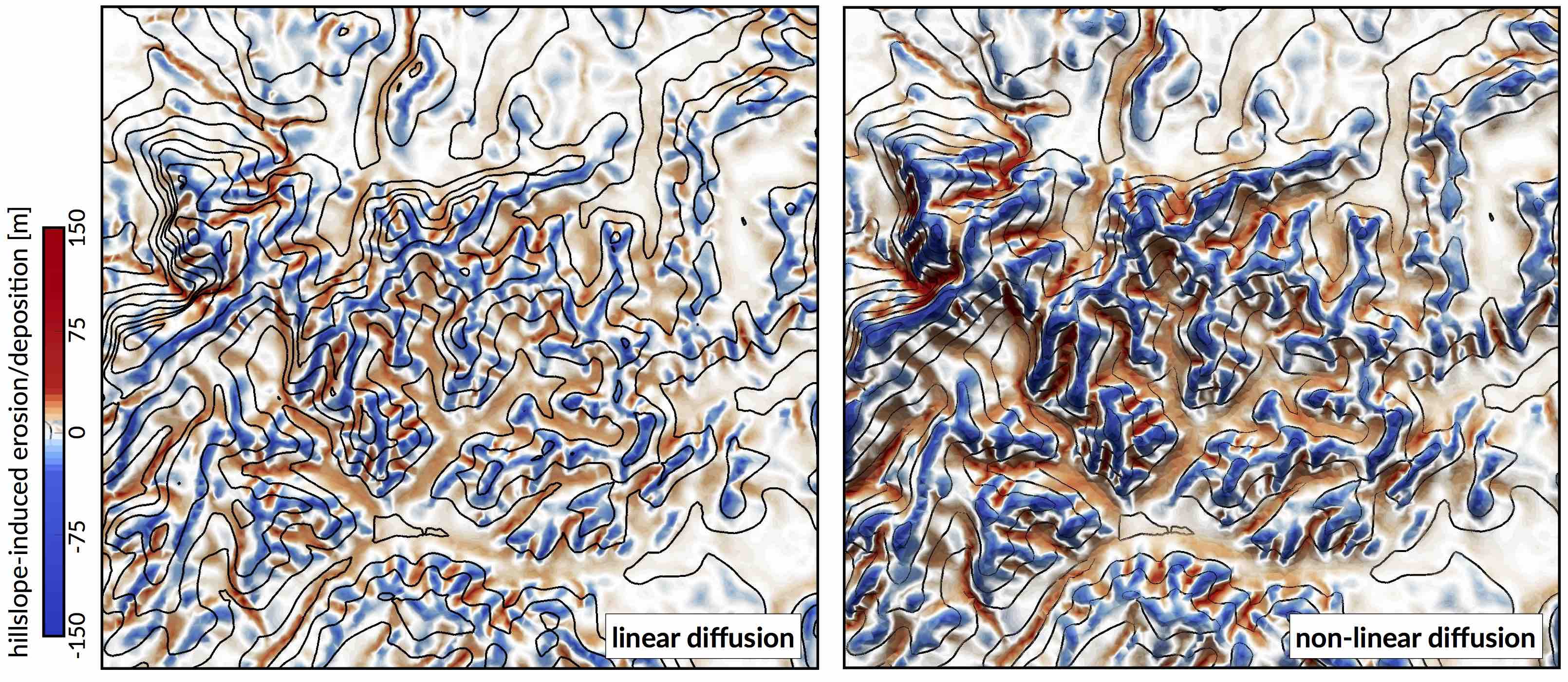
Hillslope processes
Along hillslopes, we assume that gravity is the main driver for transport and state that the flux of sediment is proportional to the gradient of topography (Fig 5).
One can choose between 2 options to simulate these processes. In the first, we use a linear diffusion law commonly referred to as soil creep :
\[\frac{\partial z}{\partial t}= \kappa_{hl} \nabla^2 z\]
in which \(\kappa_{hl}\) is the diffusion coefficient and can be defined with different values for the marine and land environments. It encapsulates, in a simple formulation, processes operating on superficial sedimentary layers. Main controls on variations of \(\kappa_{hl}\) include substrate, lithology, soil depth, climate and biological activity.
Field evidence, however, suggests that the linear diffusion approximation (Eq 10) is only rarely appropriate . Instead, Andrews and Bucknam and Roering et al. proposed a nonlinear formulation of diffusive hillslope transport, assuming that flux rates increase to infinity if slope values approach a critical slope \(S_c\). This alternative formulation is available as a second option and takes the following form in our model:
\[\frac{\partial z}{\partial t}= \nabla \cdot \frac{\kappa_{hn} \nabla z}{1-(|\nabla z|/S_c)^2}\]
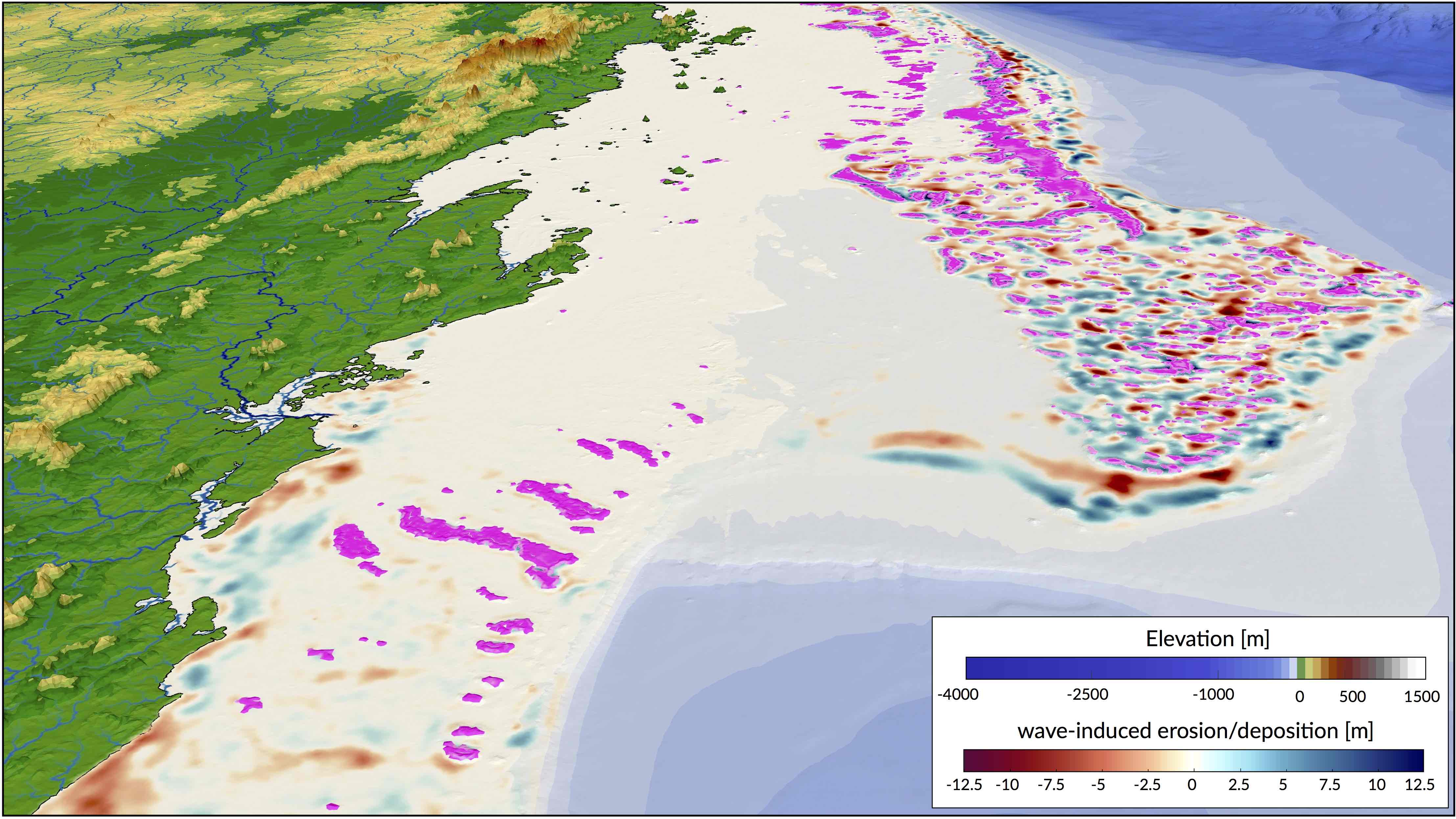
Wave-induced longshore drift
We adopt the most basic known principles of wave motion, i.e., the linear wave theory . Wave celerity \(c\) is governed by:
\[c=\sqrt{\frac{g}{\kappa}\tanh{\kappa d}}\]
where \(g\) is the gravitational acceleration, \(\kappa\) the radian wave number (equal to \(2\pi/L\), with \(L\) the wave length), and \(d\) is the water depth. In deep water, the celerity is dependent only on wave length (\(\sqrt{gL/2\pi}\)); in shallow water, it depends on depth (\(\sqrt{gd}\)). From wave celerity and wave length, we calculate wave front propagation (including refraction) using the Huygens principle . From this, we deduce the wave travel time and define wave directions from lines perpendicular to the wave front. Wave height (\(H\)) is then calculated along wave front propagation. The algorithm takes into account wave energy dissipation in shallow environment as well as wave-breaking conditions.
Wave-induced sediment transport is related to the maximum bottom wave-orbital velocity \(u_{w,b}\). Assuming the linear shallow water approximation , its expression is simplified as:
\[u_{w,b}=(H/2)\sqrt{g/d}\]
Under pure waves (i.e., no superimposed current), the wave-induced bed shear stress \(\tau_w\) is typically defined as a quadratic bottom friction :
\[\tau_{w}=\frac{1}{2}\rho f_w u_{w,b}^2\]
with \(\rho\) the water density and \(f_w\) is the wave friction factor. Considering that the wave friction factor is only dependent of the bed roughness \(k_b\) relative to the wave-orbital semi-excursion at the bed \(A_b\) , we define:
\[f_w=1.39\left(A_b/k_b\right)^{-0.52}\]
where \(A_b=u_{w,b}T/2\pi\) and \(k_b=2\pi d_{50} / 12\), with \(d_{50}\) median sediment grain-size at the bed and \(T\) the wave period.
For each wave condition, the wave transformation model computes wave characteristics and the induced bottom shear stress. These parameters are subsequently used to evaluate the long-term sediment transport active over the simulated region.
We assume that flow circulation is mainly driven by waves and other processes such as coastal upwelling, tidal, ocean or wind-driven currents are ignored. The proposed method consists in producing snapshots of wave-driven circulation distribution resulting from series of deep-water wave scenarios by computing time-averaged longshore current. In nearshore environments, longshore current runs parallel to the shore and significantly contributes to sediment transport . The longshore current velocity (\(\vec{v_l}\)) in the middle of the breaking zone is defined by Komar & Miller :
\[\vec{v_l} = \kappa_l u_{w,b} cos(\theta) sin(\theta) \vec{k}\]
with \(\theta\) the angle of incidence of the incoming waves, \(\kappa_l\) a scaling parameter and \(\vec{k}\) the unit vector parallel to the breaking depth contour.
In regions where wave-induced shear stress (Eq 14) is greater than the critical shear stress derived from the Shields parameter (\(\tau_c = \theta_c gd_{50}(\rho_s-\rho_w)\)), bed sediments are entrained. The erosion thickness \(h_e\) is limited to the top sedimentary layer and for simplicity is assumed to follow a logarithmic form :
\[h_e = C_e \ln(\tau_w/\tau_c) \text{ where } \tau_w > \tau_c\]
where \(C_e\) is an entrainment coefficient controlling the relationship between shear stress and erosion rate . Once entrained, sediments are transported following the direction of longshore currents and are deposited in regions where \(\tau_{w}<\tau_c\) (Fig 6).
Carbonate production
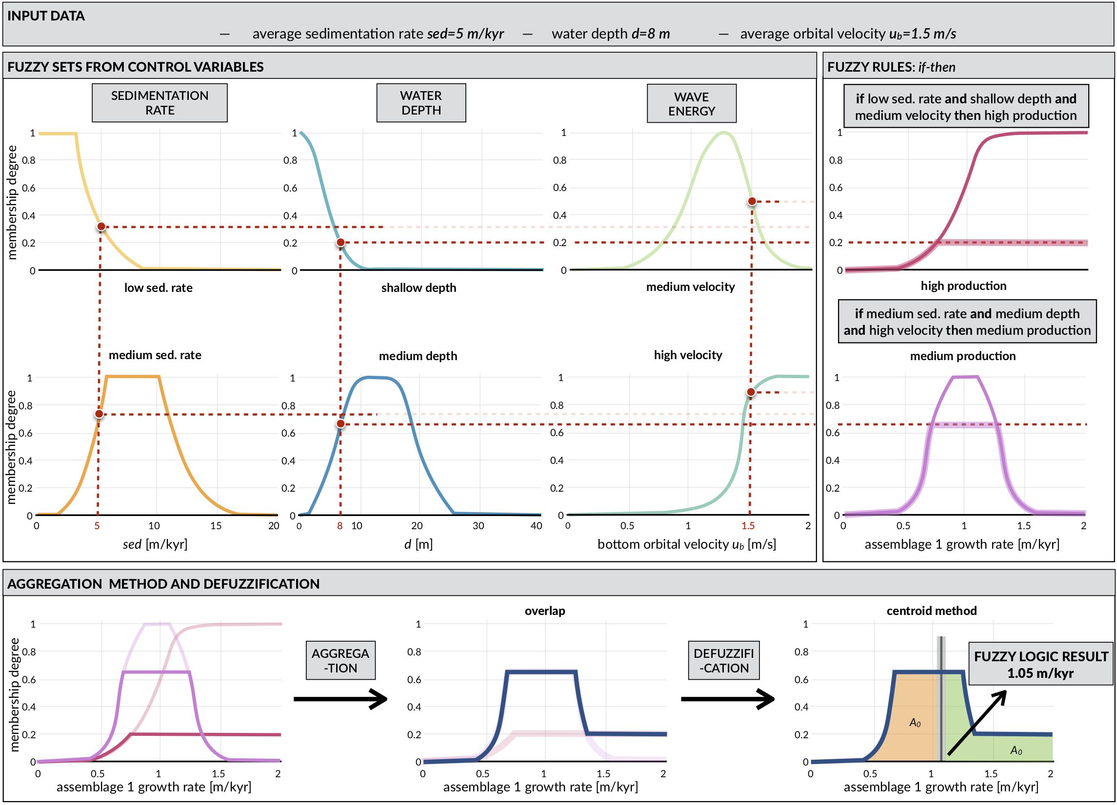
The organisation of coral reef systems is known to be large and complex and we are still limited in our understanding of their temporal and spatial evolution . Additionally, most datasets of carbonate systems are often linguistic, context-dependent, and based on measurements with large uncertainties. Alternative approaches, such as fuzzy logic or cellular automata algorithms, have proven to be viable options to simulate these types of system . Fuzzy logic methods are able to create logical propositions from qualitative data by using linguistic logic rules and fuzzy sets . These fuzzy sets are defined with continuous boundaries rather than crisp discontinuous ones often used in conventional methods .
Based on a fuzzy logic approach, carbonate system evolution in badlands is driven entirely by a set of rules whose variables are fully adjustable. The utility and effectiveness of the approach is mostly based on the user’s understanding of the modelled carbonate system . The technique is specifically useful to understand how particular variable, in isolation or in combination with other factors, influences carbonate depositional geometries and reef adaptation (Fig 7).
Here, carbonate growth depends on three types of control variables: depth (or accommodation space), wave energy (derived from ocean bottom orbital velocity) and sedimentation rate. For each of these variables, one can define a range of fuzzy sets using membership functions . A membership function is a curve showing the degree of truth (i.e. ranging between 0 and 1) of membership in a particular fuzzy set (Fig 7). These curves can be simple triangles, trapezoids, bell-shaped curves, or have more complicated shapes as shown in Fig 7.
Production of any specific coral assemblage is then computed from a series of fuzzy rules. A fuzzy rule is a logic if-then rule defined from the fuzzy sets . Here, the combination of the fuzzy sets in each fuzzy rule is restricted to the and operator. The amalgamation of competing fuzzy rules is usually referred to as a fuzzy system. Summation of multiple rules from the fuzzy system by truncation of the membership functions produces a fuzzy answer in the form of a membership set (Fig 7). The last step consists in computing a single number for this fuzzy set through defuzzification . In our approach, the centroid (centre of gravity) for the area below the membership set is taken as the defuzzified output value. The process returns a crisp value of coral assemblage growth on each cell of the simulated region (Fig 6).
Extrinsic forcing
Over geological time scales, sediment transport from source to sink is primarily controlled by climate, tectonics and eustatism (Fig 1). In badlands, the following set of external forcing mechanisms could be considered:
- sea-level fluctuations,
- subsidence, uplift and horizontal displacements,
- rainfall regimes and
- boundary wave conditions.
Tectonic forcing is driven by series of temporal maps. Each map can have variable spatial cumulative displacements making it possible to simulate complex 3D tectonic evolution with both vertical (uplift and subsidence) and horizontal directions. When 3D deformations is imposed, the model uses the node refinement technique proposed by Thieulot et al. . The geometry of the surface is first advected by tectonic forces before being modified by surface processes. Due to tectonic advection, the density of the nodes evolves over time, which could lead to unbalanced resolutions with places showing either rarefaction or accumulation of nodes. To limit this effect, the advected surface is modified by adding or removing nodes to ensure homogeneous nodes distribution.
Sea-level elevation through time can be imposed from either a published eustatic curve or directly defined by the user.
| Temporal variations in precipitation |
Precipitation might be applied either as a constant values (metres per year) or a set of maps representing spatially changing rainfall regimes. In addition, to account for the interactions between rainfall and topography, the option is given to use the orographic precipitation linear model from Smith & Barstad . As an example, the coupled evolution of precipitation patterns and topography can be use to quantify the relative importance of climate, erosion and tectonic in mountain geomorphology.
To evaluate marine sediment transport over several thousands of years, the approach taken here relies on stationary representation of prevailing fair-weather wave conditions. The wave transformation model is generally performed for time intervals varying from 5 to 50 years. The aim is to simulate realistic wave fields by imposing a sequence of wave forcing conditions. At any given time interval, we define a percentage of activity for each deep-water wave conditions as well as the significant wave height. Then, the bathymetry is used to compute associated wave parameters.
Important
The forcing mechanisms described above will directly control the evolution of sediment transport, associated stratal architecture as well as carbonate production.